Python 3home |
Advanced Python
davidbpython.com
Algorithmic Complexity Analysis and "Big O"
Introduction: the Coding Interview
Coding interviews follow a consistent pattern of evaluation and success criteria.
What interviewers are considering: Analytical Skills: how easily, how well and how efficiently did you solve a coding challenge? Coding Skills: how clear and well organized was your code, did you use proper style, and did you consider potential errors? Technical knowledge / computer science fundamentals: how familiar are you with the technologies relevant to the position? Experience: have you built interesting projects or solved interesting problems, and have you demonstrated passion for what you are doing? Culture Fit: can you tell a joke, and can you take one? Seriously, does your personality fit in with the office or team culture? The interview process: The phone screen: 1-2 calls focusing first on your personality and cultural fit, and then on your technical skills. Some phone screens include a coding interview. The take-home exam: a coding problem that may or may not be timed. Your code may be evaluated for a number of factors: good organization and style, effective solution, efficient algorithm. The in-person interview: 1 or more onsite interviews with engineers, team lead and/or manager. If the office is out of town you may even fly there (at company's expense). Many onsite interviews are full-day, in which several stakeholders interview you in succession. The whiteboard coding interview: For various reasons most companies prefer that you write out code on a whiteboard. You should consider practicing coding challenges on a whiteboard if only just to get comfortable with the pen. Writing skills are important, particularly when writing a "pretty" (i.e., without brackets) language like Python.
Introduction: Algorithmic Complexity Analysis
Algorithms can be analyzed for efficiency based on how they respond to varying amounts of input data.
Algorithm: a block of code designed for a particular purpose. You may have heard of a sort algorithm, a mapping or filtering algorithm, a computational algorithm; Google's vaunted search algorithm or Facebook's "feed" algorithm; all of these refer to the same concept -- a block of code designed for a particular purpose. Any block of code is an algorithm, including simple ones. Since algorithms can be well designed or poorly designed, time efficient or inefficient, memory efficient or inefficient, it becomes a meaningful discipline to analyze the efficiency of one approach over another. Some examples are taken from the premier text on interview questions and the coding interview process, Cracking the Coding Interview, by Gayle Laakmann McDowell. Several of the examples and information in this presentation can be found in a really clear textbook on the subject, Problem Solving with Algorithms and Data Structures, also available as a free PDF.
The order ("growth rate") of a function
The order describes the growth in steps of a function as the input size grows.
A "step" can be seen as any individual statement, such as an assignment or a value comparison. Depending on its design, an algorithm may take take the same number of steps no matter how many elements are passed to input ("constant time"), an increase in steps that matches the increase in input elements ("linear growth"), or an increase that grows faster than the increase in input elements ("logarithmic", "linear logarithmic", "quadratic", etc.). Order is about growth of number of steps as input size grows, not absolute number of steps. Consider this simple file field summer. How many more steps for a file of 5 lines than a file of 10 lines (double the growth rate)? How many more for a file of 1000 lines?
def sum_fieldnum(filename, fieldnum, delim):
    this_sum = 0.0
    fh = open(filename)
    for line in fh:
        items = line.split(delim)
        value = float(items[fieldnum])
        this_sum = this_sum + value
    fh.close()
    return this_sum
Obviously several steps are being taken -- 5 steps that don't depend on the data size (initial assignment, opening of filehandle, closing of filehandle and return of summed value) and 3 steps taken once for each line of the file (split the line, convert item to float, add float to sum) Therefore, with varying input file sizes, we can calulate the steps:
   5 lines:  5 + (3 * 5),    or 5 + 15,   or 20 steps
  10 lines:  5 + (3 * 10),   or 5 + 30,   or 35 steps
1000 lines:  5 + (3 * 1000), or 5 + 3000, or 3005 steps
As you can see, the 5 "setup" steps become trivial as the input size grows -- it is 25% of the total with a 5-line file, but 0.0016% of the total with a 1000-line file, which means that we should consider only those steps that are affected by input size -- the rest are simply discarded from analysis.
A simple algorithm: sum up a list of numbers
Here's a simple problem that will help us understand the comparison of algorithmic approaches.
It also happens to be an interview question I heard when I was shadowing an interview: Given a maximum value n, sum up all values from 0 to the maximum value. "range" approach:
def sum_of_n_range(n):
    total = 0
    for i in range(1,n+1):
        total = total + i
    return total

print(sum_of_n_range(10))
"recursive" approach:
def sum_of_n_recursive(total, count, this_max):
    total = total + count
    count += 1
    if count > this_max:
        return total
    return sum_of_n_recursive(total, count, this_max)

print(sum_of_n_recursive(0, 0, 10))
"formula" approach:
def sum_of_n_formula(n):
    return (n * (n + 1)) // 2

print(sum_of_n_formula(10))
We can analyze the respective "order" value for each of these functions by comparing its behavior when we pass it a large vs. a small value. We count each statement as a "step". The "range" solution begins with an assignment. It loops through each consecutive integer between 1 and the maximum value. For each integer it performs a sum against the running sum, then returns the final sum. So if we call sum_of_n_range with 10, it will perform the sum (total + i) 10 times. If we call it with 1,000,000, it will perform the sum 1,000,000 times. The increase in # of steps increases in a straight line with the # of values to sum. We call this linear growth. The "recursive" solution calls itself once for each value in the input. This also requires a step increase that follows the increase in values, so it is also "linear". The "formula" solution, on the other hand, arrives at the answer through a mathematic formula. It performs an addition, multiplication and division of values, but the computation is the same regardless of the input size. So whether 10 or 1,000,000, the number of steps is the same. This is known as constant time.
"Big O" notation
The order of a function (the growth rate of the function as its input size grows) is expressed with a mathematical expression colloquially referred to as "Big O".
Common function notations for Big O
Here is a table of the most common growth rates, both in terms of their O notation and English names:
"O" Notation Name
O(1) Constant
O(log(n)) Logarithmic
O(n) Linear
O(n * log(n)) Log Linear
O(n²) Quadratic
O(n³) Cubic
O(2^n) (2 to the power of n) Exponential
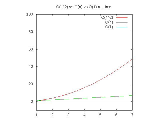
Here's a graph of the constant, linear and exponential growth rates:
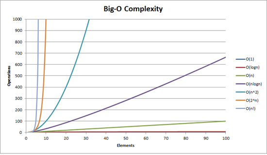
 Here's a graph of the other major scales. You can see that at this scale, "constant time" and "logarithmic" seem very close:
Here is the wiki page for "Big O":
https://en.wikipedia.org/wiki/Big_O_notation
Constant time: O(1)
A function that does not grow in steps or operations as the input size grows is said to be running at constant time.
def sum_of_n_formula(n):
    return (n * (n + 1)) // 2

print(sum_of_n_formula(10))
That is, no matter how big n gets, the number of operations stays the same. "Constant time" growth is noted as O(1).
Linear growth: O(n)
The growth rate for the "range" solution to our earlier summing problem (repeated below) is known as linear growth.
With linear growth, as the input size (or in this case, the integer value) grows, the number of steps or operations grows at the same rate:
def sum_of_n_range(n):
    the_sum = 0
    for i in range(1,n+1):
        the_sum = the_sum + i
    return the_sum

print(sum_of_n_range(10))
Although there is another operation involved (the assignment of the_sum to 0), this additional step becomes trivial as the input size grows. We tend to ignore this step in our analysis because we are concerned with the function's growth, particularly as the input size becomes large. Linear growth is noted as O(n) where again, n is the input size -- growth of operations matching growth of input size.
Logarithmic growth: O(log(n))
A logarithm is an equation used in algebra. We can consider a log equation as the inverse of an exponential equation:
b^c = a ("b to the power of c equals a")
10³ = 1000 ## 10 cubed == 1000
is considered equivalent to: logba = c ("log with base b and value a equals c")
log101000 = 3
A logarithmic scale is a nonlinear scale used to represent a set of values that appear on a very large scale and a potentially huge difference between values, with some relatively small values and some exponentially large values. Such a scale is needed to represent all points on a graph without minimizing the importance of the small values. Common uses of a logarithmic scale include earthquake magnitude, sound loudness, light intensity, and pH of solutions. For example, the Richter Scale of earthquake magnitude grows in absolute intensity as it moves up the scale -- 5.0 is 10 times that of 4.0; 6.0 is 10 times that of 5.0; 7.0 is 10 times that of 6.0, etc. This is known as a base 10 logarithmic scale. In other words, a base 10 logarithmic scales runs as:
1, 10, 100, 1000, 10000, 100000, 1000000
Logarithms in Big O notation However, the O(log(n)) ("Oh log of n") notation refers to a base 2 progression - 2 is twice that of 1, 3 is twice that of 2, etc. In other words, a base 2 logarithmic scale runs as:
1, 2, 4, 8, 16, 32, 64
A classic binary search algorithm on an ordered list of integers is O(log(n)). You may recognize this as the "guess a number from 1 to 100" algorithm from one of the extra credit assignments.
def binary_search(alist, item):
    first = 0
    last = len(alist)-1
    found = False

    while first<=last and not found:
        midpoint = (first + last)//2
        if alist[midpoint] == item:
            found = True
        else:
            if item < alist[midpoint]:
                last = midpoint-1
            else:
                first = midpoint+1

    return found

print(binary_search([1, 3, 4, 9, 11, 13], 11))

print(binary_search([1, 2, 4, 9, 11, 13], 6))
The assumption is that the search list is sorted. Note that once the algorithm decides whether the search integer is higher or lower than the current midpoint, it "discards" the other half and repeats the binary searching on the remaining values. Since the number of loops is basically n/2/2/2/2, we are looking at a logarithmic order. Hence O(log(n))
Linear logarithmic growth: O(n * log(n))
The basic approach of a merge sort is to halve it; loop through half of it; halve it again.
def merge_sort(a_list):
    print(("Splitting ", a_list))
    if len(a_list) > 1:
        mid = len(a_list) // 2      # (floor division, so lop off any remainder)
        left_half = a_list[:mid]
        right_half = a_list[mid:]

        merge_sort(left_half)
        merge_sort(right_half)

        i = 0
        j = 0
        k = 0

        while i < len(left_half) and j < len(right_half):
            if left_half[i] < right_half[j]:
                a_list[k] = left_half[i]
                i = i + 1
            else:
                a_list[k] = right_half[j]
                j = j + 1
            k = k + 1

        while i < len(left_half):
                a_list[k] = left_half[i]
                i = i + 1
                k = k + 1

        while j < len(right_half):
                a_list[k] = right_half[j]
                j = j + 1
                k = k + 1
    print(("Merging ", a_list))

a_list = [54, 26, 93, 17, 77, 31, 44, 55, 20]
merge_sort(a_list)
print(a_list)
The output of the above can help us understand what portions of the unsorted list are being managed:
('Splitting ', [54, 26, 93, 17, 77, 31, 44, 55, 20])
('Splitting ', [54, 26, 93, 17])
('Splitting ', [54, 26])
('Splitting ', [54])
('Merging ', [54])
('Splitting ', [26])
('Merging ', [26])
('Merging ', [26, 54])
('Splitting ', [93, 17])
('Splitting ', [93])
('Merging ', [93])
('Splitting ', [17])
('Merging ', [17])
('Merging ', [17, 93])
('Merging ', [17, 26, 54, 93])
('Splitting ', [77, 31, 44, 55, 20])
('Splitting ', [77, 31])
('Splitting ', [77])
('Merging ', [77])
('Splitting ', [31])
('Merging ', [31])
('Merging ', [31, 77])
('Splitting ', [44, 55, 20])
('Splitting ', [44])
('Merging ', [44])
('Splitting ', [55, 20])
('Splitting ', [55])
('Merging ', [55])
('Splitting ', [20])
('Merging ', [20])
('Merging ', [20, 55])
('Merging ', [20, 44, 55])
('Merging ', [20, 31, 44, 55, 77])
('Merging ', [17, 20, 26, 31, 44, 54, 55, 77, 93])
[17, 20, 26, 31, 44, 54, 55, 77, 93]
Here's an interesting description comparing O(log(n)) to O(n * log(n)):
log(n) is proportional to the number of digits in n.

n * log(n) is n times greater.

Try writing the number 1000 once versus writing it one thousand times.
The first takes O(log(n)) time, the second takes O(n * log(n) time.

Now try that again with 6700000000. Writing it once is still trivial.
Now try writing it 6.7 billion times.
We'll check back in a few years to see your progress.
Quadratic growth: O(n^2;)
O(n²) growth can best be described as "for each element in the sequence, loop through the sequence". This is why it's notated as n².
def all_combinations(the_list):
   results = []
   for item in the_list:
       for inner_item in the_list:
           results.append((item, inner_item))
   return results

print(all_combinations(['a', 'b', 'c', 'd', 'e', 'f', 'g']))
Clearly we're seeing n * n, so 49 individual tuple appends.
[('a', 'a'), ('a', 'b'), ('a', 'c'), ('a', 'd'), ('a', 'e'), ('a', 'f'),
 ('a', 'g'), ('b', 'a'), ('b', 'b'), ('b', 'c'), ('b', 'd'), ('b', 'e'),
 ('b', 'f'), ('b', 'g'), ('c', 'a'), ('c', 'b'), ('c', 'c'), ('c', 'd'),
 ('c', 'e'), ('c', 'f'), ('c', 'g'), ('d', 'a'), ('d', 'b'), ('d', 'c'),
 ('d', 'd'), ('d', 'e'), ('d', 'f'), ('d', 'g'), ('e', 'a'), ('e', 'b'),
 ('e', 'c'), ('e', 'd'), ('e', 'e'), ('e', 'f'), ('e', 'g'), ('f', 'a'),
 ('f', 'b'), ('f', 'c'), ('f', 'd'), ('f', 'e'), ('f', 'f'), ('f', 'g'),
 ('g', 'a'), ('g', 'b'), ('g', 'c'), ('g', 'd'), ('g', 'e'), ('g', 'f'),
 ('g', 'g')]
Exponential Growth: O(2^n)
Exponential denotes an algorithm whose growth doubles with each additon to the input data set.
One example would be the recursive calculation of a Fibonacci series
def fibonacci(num):
    if num <= 1:
        return num
    return fibonacci(num - 2) + fibonacci(num - 1)

for i in range(10):
    print(fibonacci(i), end=' ')
Best Case, Expected Case, Worst Case
Case analysis considers the outcome if data is ordered conveniently or inconveniently.
For example, given a test item (an integer), search through a list of integers to see if that item's value is in the list. Sequential search (unsorted):
def sequential_search(a_list, item):
    pos = 0
    found = False
    for test_item in a_list:
        if test_item == item:
            found = True
            break
    return found

test_list = [1, 2, 32, 8, 17, 19, 42, 13, 0]
print(sequential_search(test_list, 2))          # best case:  found near start
print(sequential_search(test_list, 17))         # expected case:  found near middle
print(sequential_search(test_list, 999))        # worst case:  not found
Analysis: 0(n) Because the order of this function is linear, or O(n), case analysis is not meaningful. Whether the best or worst case, the rate of growth is the same. It is true that "best case" results in very few steps taken (closer to O(1)), but that's not helpful in understanding the function. When case matters Case analysis comes into play when we consider that an algorithm may seem to do well with one dataset (best case), not as well with another dataset (expected case), and poorly with a third dataset (worst case). A quicksort picks a random pivot, divides the unsorted list at that pivot, and sorts each sublist by selecting another pivot and dividing again.
def quick_sort(alist):
   """ initial start """

   quick_sort_helper(alist, 0, len(alist) - 1)


def quick_sort_helper(alist, first_idx, last_idx):
   """  calls partition() and retrieves a split point,
        then calls itself with '1st half' / '2nd half' indices """

   if first_idx < last_idx:
       splitpoint = partition(alist, first_idx, last_idx)

       quick_sort_helper(alist, first_idx, splitpoint - 1)
       quick_sort_helper(alist, splitpoint + 1, last_idx)


def partition(alist, first, last):
   """ main event:  sort items to either side of a pivot value """

   pivotvalue = alist[first]   # very first item in the list is "pivot value"

   leftmark = first + 1
   rightmark = last

   done = False
   while not done:

       while leftmark <= rightmark and alist[leftmark] <= pivotvalue:
           leftmark = leftmark + 1

       while alist[rightmark] >= pivotvalue and rightmark >= leftmark:
           rightmark = rightmark - 1

       if rightmark < leftmark:
           done = True
       else:
           # swap two items
           temp = alist[leftmark]
           alist[leftmark] = alist[rightmark]
           alist[rightmark] = temp

   # swap two items
   temp = alist[first]
   alist[first] = alist[rightmark]
   alist[rightmark] = temp

   return rightmark


alist = [54, 26, 93, 17, 77]
quick_sort(alist)
print(alist)
Best case: all elements are equal -- sort traverses the elements once (O(n)) Worst case: the pivot is the biggest element in the list -- each iteration just works on one item at a time (O(n²)) Average case: the pivot is more or less in the middle -- O(n * log(n))
"order" analysis example
Let's take an arbitrary example to analyze. This algorithm is working with the variable n -- we have not defined n because it represents the input data, and our analysis will ask: how does the time needed change as n grows? However, we can assume that n is a sequence.
a = 5                   # count these up:
b = 6                   # 3 statements
c = 10

for k in range(n):
    w = a * k + 45      # 2 statements:
    v = b * b           # but how many times
                        # will they execute?

for i in range(n):
    for j in range(n):
        x = i * i       # 3 statements:
        y = j * j       # how many times?
        z = i * j

d = 33                  # 1 statement
* We can count assignment statements that are executed once: there are 4 of these. * The 2 statements in the first loop are each being executed once for each iteration of the loop -- and it is iterating n times. So we call this 2n. * The 3 statements in the second loop are being executed n times * n times (a nested loop of range(n). We can call this n² ("n squared"). So the order equation can be expressed as 4 + 2n + n² eliminating the trivial factors However, remember that this analysis describes the growth rate of the algorithm as input size n grows very large. As n gets larger, the impact of 4 and of 2n become less and less significant compared to n²; eventually these elements become trivial. So we eliminate the lessor factors and pay attention only to the most significant -- and our final calculation is O(n²).
Big O Analysis: rules of thumb
Here are some practical ways of thinking, courtesy of The Idiot's Guide to Big O
* Does it have to go through the entire list? There will be an n in there somewhere. * Does the algorithms processing time increase at a slower rate than the size of the data set? Then there's probably a log(n) in there. * Are there nested loops? You're probably looking at n^2 or n^3. * Is access time constant irrelevant of the size of the dataset?? O(1)
More Big O recursion examples
These were adapted from a stackoverflow question. Just for fun(!) these are presented without answers; answers on the next page.
def recurse1(n):
    if n <= 0:
        return 1
    else:
        return 1 + recurse1(n-1)
def recurse2(n):
    if n <= 0:
        return 1
    else:
        return 1 + recurse2(n-5)
def recurse3(n):
    if n <= 0:
        return 1
    else:
        return 1 + recurse3(n / 5)
def recurse4(n, m, o):
    if n <= 0:
        print('{}, {}'.format(m, o))
    else:
        recurse4(n-1, m+1, o)
        recurse4(n-1, m, o+1)
def recurse5(n):
    for i in range(n)[::2]:       # count to n by 2's (0, 2, 4, 6, 7, etc.)
        pass
    if n <= 0:
        return 1
    else:
        return 1 + recurse5(n-5)
More Big O recursion examples: analysis
def recurse1(n):
    if n <= 0:
        return 1
    else:
        return 1 + recurse1(n-1)
This function is being called recursively n times before reaching the base case so it is O(n) (linear)
def recurse2(n):
    if n <= 0:
        return 1
    else:
        return 1 + recurse2(n-5)
This function is called n-5 for each time, so we deduct five from n before calling the function, but n-5 is also O(n) (linear).
def recurse3(n):
    if n <= 0:
        return 1
    else:
        return 1 + recurse3(n // 2)
This function is log(n), for every time we divide by 2 before calling the function.
def recurse4(n, m, o):
    if n <= 0:
        print('{}, {}'.format(m, o))
    else:
        recurse4(n-1, m+1, o)
        recurse4(n-1, m, o+1)
In this function it's O(2^n), or exponential, since each function call calls itself twice unless it has been recursed n times.
def recurse5(n):
    for i in range(n)[::2]:       # count to n by 2's (0, 2, 4, 6, 7, etc.)
        pass
    if n <= 0:
        return 1
    else:
        return 1 + recurse5(n-5)
The for loop takes n/2 since we're increasing by 2, and the recursion takes n-5 and since the for loop is called recursively, the time complexity is in (n-5) * (n/2) = (2n-10) * n = 2n^2- 10n, so O(n²)
Efficiency of core Python Data Structure Algorithms
note: "k" is the list being added/concatenated/retrieved
| List | |
| Operation | Big-O Efficiency |
|---|---|
| index[] | O(1) |
| index assignment | O(1) |
| append | O(1) |
| pop() | O(1) |
| pop(i) | O(n) |
| insert(i,item) | O(n) |
| del operator | O(n) |
| iteration | O(n) |
| contains (in) | O(n) |
| get slice [x:y] | O(k) |
| del slice | O(n) |
| set slice | O(n + k) |
| reverse | O(n) |
| concatenate | O(k) |
| sort | O(n * log(n) |
| multiply | O(nk) |
| Dict | |
| Operation | Big-O Efficiency (avg.) |
|---|---|
| copy | O(n) |
| get item | O(1) |
| set item | O(1) |
| delete item | O(1) |
| contains (in) | O(1) |
| iteration | O(n) |
Common Algorithms Organized by Efficiency
O(1) time 1. Accessing Array Index (int a = ARR[5]) 2. Inserting a node in Linked List 3. Pushing and Poping on Stack 4. Insertion and Removal from Queue 5. Finding out the parent or left/right child of a node in a tree stored in Array 6. Jumping to Next/Previous element in Doubly Linked List and you can find a million more such examples... O(n) time 1. Traversing an array 2. Traversing a linked list 3. Linear Search 4. Deletion of a specific element in a Linked List (Not sorted) 5. Comparing two strings 6. Checking for Palindrome 7. Counting/Bucket Sort and here too you can find a million more such examples.... In a nutshell, all Brute Force Algorithms, or Noob ones which require linearity, are based on O(n) time complexity O(log(n)) time 1. Binary Search 2. Finding largest/smallest number in a binary search tree 3. Certain Divide and Conquer Algorithms based on Linear functionality 4. Calculating Fibonacci Numbers - Best Method The basic premise here is NOT using the complete data, and reducing the problem size with every iteration O(n * log(n)) time 1. Merge Sort 2. Heap Sort 3. Quick Sort 4. Certain Divide and Conquer Algorithms based on optimizing O(n^2) algorithms The factor of 'log(n)' is introduced by bringing into consideration Divide and Conquer. Some of these algorithms are the best optimized ones and used frequently. O(n^2) time 1. Bubble Sort 2. Insertion Sort 3. Selection Sort 4. Traversing a simple 2D array These ones are supposed to be the less efficient algorithms if their O(n * log(n)) counterparts are present. The general application may be Brute Force here.