Python 3home |
All Slides on One Page
Python Intermediate Features
The Introduction to Python course that many of you have taken focused on core features that were considered essential to performing core tasks. However there were a number of features that are still considered "introductory", but were deliberately omitted to help maintain focus on these core features. This slide deck is devoted to bringing you up to speed on these basic features.
dict .get()
Safely get a value from a dictionary without raising a KeyError if the key doesn’t exist.
The .get() method returns the value for a given key in a dictionary. If the key is not found, it returns a default value (or None if no default is given) instead of raising an error.
data = {"a": 1, "b": 2}

val1 = data.get("a")        # int, 1
val2 = data.get("c")        # None
val3 = data.get("c", 0)     # int, 0
We use `.get()` when we want to access dictionary values safely without risking a `KeyError`. It's especially useful when working with user input, optional keys, or data from external sources like APIs.
dict .items()
Retrieve all key-value pairs from a dictionary as (key, value) tuples for iteration or inspection.
The .items() method returns a view of a dictionary’s key-value pairs. Each pair is returned as a tuple.
data = {"a": 1, "b": 2}

for key, value in data.items():
    print(key, value)             # a 1
                                  # b 2
We use .items() when we want to loop through both keys and values in a dictionary at the same time. It's commonly used in for loops to process each entry efficiently.
The 'with' context with objects
Ensure proper acquisition and release of resources, like files or network connections.
The with statement in Python is used to automatically close a file. The file object is actually programmed to close itself as soon as execution leaves the with block.
with open("file.csv", "r") as fh:
    for line in fh:
        print(line)
We use with to automatically handle opening and closing resources, even if an error occurs during use. This makes code cleaner and less error-prone.
with is especially helpful when working with database connections. Database connections are important to release quickly, because they are often shared and in short supply.
import sqlite3

with sqlite3.connect("example.db") as conn:
    cursor = conn.cursor()
    cursor.execute("SELECT * FROM users")
As with the file, the connection object conn is programmed to closed automatically when exiting the block ends, even if an error occurs.
range()
Generate a sequence of integers for iteration, usually in loops.
range() generates a sequence of numbers, often used in for loops.
for i in range(3):
    print(i)           # 0
                       # 1
                       # 2
You can also use the list() function to preserve the numbers:
nums = list(range(3)) # [0, 1, 2]
The range of numbers doesn't need to start at 0:
for i in range(1, 5):
    print(i)            # 1
                        # 2
                        # 3
                        # 4
Note that the upper bound is non-inclusive, the same as with list slices.
A third argument, the step, allows for 'skipping' of nubmers through the count:
for i in range(1, 11, 3):
    print(i)               # 1
                           # 4
                           # 7
                           $ 10
enumerate()
Loop over an iterable while keeping track of the index automatically.
enumerate() adds a counter to an iterable and returns each item as (index, value) pairs. It’s often used in loops when both item and position are needed.
items = ["a", "b", "c"]

for index, value in enumerate(items):
    print(index, value)                # 0 a
                                       # 1 b
                                       # 2 c
We use enumerate() to avoid manually tracking indexes when looping. It keeps code cleaner and less error-prone.
enumerate() can be usefully used with a file, to number the lines:
with open("example.txt", "r") as f:
    for line_num, line in enumerate(f, start=1):
        print(f"{line_num}: {line.strip()}")
Note the start=1 argument, which starts the counting at a number of your choice.
The date, datetime and timedelta objects
Date calculations are easily managed with these objects.
The date object represents a date.
from datetime import date, timedelta

today = date.today()           # date object representing today (2025-03-26)
three_days = timedelta(days=3)

then = today + three_days

print(then)                    # date(2025, 3, 29)
This can help with calculations that may be a bit more complex - handling whether months have 28, 29, 30 or 31 days.
The datetime object represents a date and time.
now = datetime.now()     # datetime object representing now (2025-03-26 5:56pm)

tomorrow = today + timedelta(days=1, hours=2)

print(tomorrow)          # datetime(2025, 03, 27, 7:56pm)
Possible arguments for timedelta():
- days
- seconds
- microseconds
- milliseconds
- minutes
- hours
- weeks
All are optional and default to 0. You can combine them as needed.
Boolean (True/False) Values
Introduction: Booleans (True/False) Values
Every object can be converted to boolean (True/False): an object is True if it is "non-zero".
counter = 5
if counter:                                            # True
    print('this int is not zero')
else:
    print('this int is zero')


mystr = ''                                             # empty string

if mystr:                                              # False
    print('this string has characters')
else:
    print('this string is empty')


var = ['a', 'b', 'c']
if var:                                                # True
    print('this container has elements')
else:
    print('this container is empty')
Summary for Object: Boolean
A boolean object can be True or False. All objects can be converted to boolean, meaning that all objects can be seen as True or False in a boolean context.
print(type(True))                                      # <type 'bool'>
print(type(False))                                     # <type 'bool'>
bool() converts objects to boolean.
print(bool(['a', 'b', 'c']))                           # True
print(bool([]))                                        # False
if and while induce the bool() conversion
So when we say if var: or while var:, we're testing if bool(var) == True, i.e., we're checking to see if the value is a True value
print(bool(5))                                         # True
print(bool(0))                                         # False
if and while induce the boolean conversion -- an object is evaluated in boolean context
mylist = [0, 0]

if mylist:                         # not empty, so True
                                   # in boolean context
    print('that list is not empty')


yourlist = [1, 2, 3]

while yourlist:                    # True as long as yourlist has elements
    x = yourlist.pop()             # remove element from the end of yourlist
    print(x)
Boolean quiz
Quiz yourself: look at the below examples and say whether the value will test as True or False in a boolean expression. Beware of tricks! Remember the rule: if it represents a 0 or empty value, it is False. Otherwise, it is True.
var   = 5
var2  = 0
var3  = -1
var4  = 0.0000000000000001
varx  = '0'
var5  = 'hello'
var6  = ""
var7  = '    '
var8  = [   ]
var9  = ['hello', 'world']
var10 = [0]
var11 = {0:0}
var12 = {}
Booleans: quiz answers
Here are the answers to the quiz.
var   = 5                       # bool(var):   True
var2  = 0                       # bool(var2):  False
var3  = -1                      # bool(var3):  True (not 0)
var4  = 0.0000000000000001      # bool(var4):  True
varx =  '0'                     # bool(varx):  True (not empty string)
var5  = 'hello'                 # bool(var5):  True
ver6  = ""                      # bool(var6):  False
var7  = '    '                  # bool(var7):  True (not empty)
var8  = [   ]                   # bool(var8):  False
var9  = ['hello', 'world']      # bool(var9):  True
var10 = [0]                     # bool(var10): True (has an element)
var11 = {0:0}                   # bool(var11): True (has a pair)
var12 = {}                      # bool(var12): False
any(), all() and "in"
any() with a sequence checks to see if any elements are True; all() asks whether they are all True; in can be used to see if a value exists in a sequence.
any(): are any of these True?
mylist = [0, 0, 5, 0]

if any(mylist):
    print('at least one item is True')
all(): are all of these True?
mylist = [5, 5, 'hello', 5.0]

if all(mylist):
    print('all items are True')
in with a list: is this value anywhere within this list?
mylist = ['highest', 'lowest']

user_choice = 'lowest'

if user_choice not in mylist:
    print('please enter "higest" or "lowest"')
Command Line: Moving Around and Executing a Script
The Command Line
The Command Line (also known as "Command Prompt" or "Terminal Prompt") gives us access to the Operating System's files and programs.
Before the graphical user interface was invented, programmers used a text-based interface called the command line to run programs and read and write files. Programmers still make heavy use of the command line because it provides a much more efficient way to communicate with the operating system than Windows Explorer or Mac Finder. It is the "power user's" way of talking to the OS. To reach the command line, you must search for and open one of these programs:
On Windows -- search for Command Prompt:
Microsoft Windows [Version 10.0.18363.1016]            # these 2 lines may not appear
(c) 2019 Microsoft Corporation. All rights reserved.

C:\Users\david>                       < -- command line
On Mac -- search for Terminal:
Last login: Thu Sep  3 13:46:14 on ttys001

Davids-MBP-3:~ david$                 < -- command line
Your command line will look similar to those shown above, but will have different names and directory paths (for example, your username instead of 'david'). After opening the command line program on your computer, note the blinking cursor: this is the OS awaiting your next command.
The Present Working Directory (pwd)
Your command line session works from one directory location at a time.
When you first launch the command line program, you are placed at a specific directory within your filesystem. We call this the "present working directory". You may "move around" the system, and when you do, your pwd will change. By default, your initial pwd is your home directory -- the directory at which all your individual files are stored. This directory is usually named after your username, and can be found at /Users/[username] or C:\Users\[username]. On Windows: Your present working directory is always displayed as the command prompt.
C:\Users\david>
On Mac:
Your present working directory can be shown by using the pwd command:
Davids-MBP-3:~ david$ pwd
/Users/david
As we move around the filesystem, we will see the present working directory change. You must always be mindful of the pwd as it is your current location and it will affect how you access other files and programs in the filesystem.
Listing files in the present working directory: 'ls' or 'dir'
We can list out the contents (files and folders) of any directory.
On Mac, use the 'ls' command to see the files and folders in the present working directory:
Davids-MBP-3:~ david$ ls

Applications
Desktop
Documents
Downloads
Dropbox
Library
Movies
Music
Public
PycharmProjects
Sites
archive
ascii_test.py
requests_demo.py
static.zip
On Windows, use the 'dir' command to see the files and folders in the present working directory:
C:\Users\david> dir

 Volume Serial Number is 0246-9FF7

 Directory of C:\Users\david

08/29/2020  11:37 AM    <DIR>          .
08/29/2020  11:37 AM    <DIR>          ..
05/29/2020  06:27 PM    <DIR>          .astropy
05/29/2020  06:35 PM    <DIR>          .config
05/29/2020  06:36 PM    <DIR>          .matplotlib
08/07/2020  10:33 AM             1,460 .python_history
08/29/2020  11:28 AM    <DIR>          3D Objects
08/29/2020  11:28 AM    <DIR>          Contacts
08/29/2020  12:50 PM    <DIR>          Desktop
08/29/2020  11:28 AM    <DIR>          Documents
09/02/2020  10:25 AM    <DIR>          Downloads
08/29/2020  11:28 AM    <DIR>          Favorites
08/29/2020  11:28 AM    <DIR>          Links
08/29/2020  11:28 AM    <DIR>          Music
08/29/2020  11:29 AM    <DIR>          OneDrive
08/29/2020  11:28 AM    <DIR>          Pictures
08/29/2020  12:46 PM    <DIR>          PycharmProjects
08/29/2020  11:28 AM    <DIR>          Saved Games
08/29/2020  11:28 AM    <DIR>          Searches
08/29/2020  11:28 AM    <DIR>          Videos
               1 File(s)          1,460 bytes
              20 Dir(s)   7,049,539,584 bytes free
Moving Around the Directory Tree With 'cd'
The 'change directory' command moves us 'up' or 'down' the tree.
To move around the filesystem (i.e. to change the present working directory), we use the cd ("change directory") command. In the examples below, note how the present working directory changes after we move.
on Mac:
Davids-MBP-3:~ david$ pwd
/Users/david

Davids-MBP-3:~ david$ cd Downloads

Davids-MBP-3:~ david$ pwd
/Users/david/Downloads
on Windows:
C:\Users\david> cd Downloads
C:\Users\david\Downloads>
So using the ls/dir command together with the cd command, we can travel from directory to directory, listing out the contents of each directory to decide where to go next (for Windows, simply substitute the dir command for ls:
Davids-MBP-3:Downloads david$ pwd
/Users/david/Downloads

Davids-MBP-3:Downloads david$ ls
python_data

Davids-MBP-3:Downloads david$ cd python_data

Davids-MBP-3:python_data david$ pwd
/Users/david/Downloads/python_data

Davids-MBP-3:python_data david$ ls
all_files
session_00_test_project
session_01_objects_types
session_02_funcs_condits_methods
session_03_strings_lists_files
session_04_containers_lists_sets
session_05_dictionaries
session_06_multis
session_07_functions_power_tools
session_08_files_dirs_stdout
session_09_funcs_modules
session_10_classes

Davids-MBP-3:python_data david$ cd session_02_funcs_condits_methods/

Davids-MBP-3:session_02_funcs_condits_methods david$ ls
warmup_exercises
inclass_exercises
notebooks_inclass_warmup
python.png

Davids-MBP-3:session_02_funcs_condits_methods david$ cd warmup_exercises/

Davids-MBP-3:warmup_exercises david$ ls
warmup_2.1.py    warmup_2.2.py    warmup_2.7.py
warmup_2.10.py   warmup_2.3.py    warmup_2.8.py
warmup_2.11.py   warmup_2.4.py    warmup_2.9.py
warmup_2.12.py   warmup_2.5.py
warmup_2.13.py   warmup_2.6.py

Davids-MBP-3:warmup_exercises david$ pwd
/Users/david/Downloads/python_data/session_02_funcs_condits_methods/warmup_exercises
The 'parent directory'
The '..' (double dot) indicates the parent and can move us one directory "up".
As you saw, we can move "down" the directory tree by using the name of the next directory -- this extends the path:
C:\Users\david> cd Downloads

C:\Users\david\Downloads> cd python_data

C:\Users\david\Downloads\python_data> cd session_02_funcs_condits_methods

C:\Users\david\Downloads\python_data\session_02_funcs_condits_methods>
But if we'd like to travel up the directory tree, we use the special .. which signifies the parent directory:
C:\Users\david\Downloads\python_data\session_02_funcs_condits_methods> cd ..

C:\Users\david\Downloads\python_data> cd ..

C:\Users\david\Downloads> cd ..

C:\Users\david>
We can also travel directly to an inner folder by using the full path:
C:\Users\david> cd python_data\session_02_funcs_condits_methods\warmup_exercises

C:\Users\david\Downloads\python_data\session_02_funcs_condits_methods\warmup_exercises>
Executing a Python Script from the Command Line
This is the "true" way to ask Python to execute our script.
Every developer should be able execute scripts through the command line, without having to use an IDE like PyCharm or Jupyter. If you are in the same directory as the script, you can execute a program by running Python and telling Python the name of the script:
On Windows:
C:\Users\david\Downloads\python_data\session_02_funcs_condits_methods> python warmup_2.1.py
On Mac:
Davids-MBP-3:warmup_exercises david$ python warmup_2.1.py
Each week we'll try to spend a few minutes traveling to and executing one or more Python programs from the command line.
Applications with Command Line Arguments
Why the Command Line is So Important
Most Python scripts are not run from an IDE.
Developers hang out on the command line for two important reasons:
- The command line features powerful utilities and commands that make working with files, directories and programs easier and more versatile
- The command line is where we usually run Python scripts and other scripts
Finding the path to Python
Your OS doesn't necessarily know where Python is until we tell it.
We should begin by seeing whether our OS already knows where python is; even if it does, we should learn the procedure for telling it where it is (for those future situations where it doesn't yet know): Windows
- Open a Command Prompt
- At the prompt type where python
- If you see a path, copy it to your clipboard and paste it into a text file.
If you don't see a path, please see the alternative approach, below. Mac
- Open a Terminal window
- At the prompt type which python
- If you see a path, copy it to your clipboard and paste it into a text file.
- If you get a "not found" message, try to determine the path as noted in the alternative approach below.
An alternative approach to determine the path to Python is to run this program from your IDE:
import sys

print(sys.executable)
Using the argparse Module to Process Command line Arguments
argparse allows us to collect and validate arguments
Many programs use command line arguments that follow the following pattern:
python myprog.py --year 2023 --factor SMB --flavors cherry vanilla chocolate
The program may require certain arguments, and show an error if they aren't passed:
python myprog.py --year 2023

usage: myprog.py [-h] -y YEAR -f FACTOR
ProgramName: error: the following arguments are required: -y/--year, -f/--factor
Such programs also offer help messages when the user typs --help as an argument:
python myprog.py --help

usage: test.py [-h] -y YEAR -f FACTOR

Reads Fama-French file to show sum of values for a selected year and selected
factor

optional arguments:
  -h, --help            show this help message and exit
  -y YEAR, --year YEAR
  -f FACTOR, --factor FACTOR
This sets up our program to use more sophisticated command line arguments. We will add the argument options in the next step.
import argparse
import os
import sys

parser = argparse.ArgumentParser(
                    prog=os.path.basename(sys.argv[0]),
                    description='Reads Fama-French file to show sum of values for a selected year and selected factor')
All of the above arguments are optional, but if used will show up in a help message if the user passes the command line argument '-h' or '--help'
Here's how we add arguments. The optional required=True causes argparse to stop the program if the argument was not passed.
parser.add_argument('-y', '--year', required=True)
parser.add_argument('-f', '--factor', required=True, choices=['Mkt-RF', 'SMB', 'HML', 'RF'])
parser.add_argument('-v', '--flavors', nargs='+')     # allow 1 or more values

args = parser.parse_args()

print(args.year)       # retrieve the value passed as <B>--year</B>
print(args.factor)     # retrieve the value passed as <B>--factor</B>
print(args.flavors)    # retrieve list of values passed as <B>--flavors</B>
Once all arguments have been added, parser.parse_args() returns an object whose attributes match the argument name. See the documentation for more options to .add_argument() that can:
- allow for multiple values to be passed as an argument (nargs=2)
- control the type allowed for an argument (type=int)
- use a default value if an argument is not passed (default=0)
- limit the possible values that can be passed as an argument (choices=['this', 'that'])
- specify a help message for an argument (help='limit data to this year')
Setting the PATH environment variable
On Windows we use the GUI; on Mac we must edit a "hidden" file.
Windows
- On the Windows taskbar, right-click the Windows icon and select System.
- In the Settings window, under Related Settings, click Advanced system settings.
- On the Advanced tab, click Environment Variables.
- Under System variables, select PATH. Click Edit to modify. (If your computer doesn't allow you to edit System variables, you may instead modify the User variables.)
- Depending on your Windows version, you may need to either edit the entire string of paths in PATH (note that the paths are separated by semicolons) or add your path to the list of paths through the GUI.
- If editing the entire string: paste your path at the start of the string of paths, and then type a semicolon to separate it from the next one.
- If you are adding your path using the GUI: with PATH highlighted, click 'New' and add the path to Python that you saved earlier. You should see the new path added to the list of variables. Then, drag the path to the top of the list.
- After modifying the environment variable, click Apply and then OK to have the change take effect.
Mac
- From the Terminal prompt, type ps -p $$
- Under CMD, if you see -bash, you're using Bash shell and should edit the ~/.bash_profile file
- If you see -zsh, you're using Z shell and should edit the ~/.zshrc file (note that your Mac may announce that "the default shell is zsh". This is just information, not an indication of which shell you are using.
- Open a Finder window to your Home directory
- Press Cmd-Shift-. (Command Key + Shift Key + period)
- Locate and edit the file determined above (.bash_profile or .zshrc). If the file doesn't exist, you should create it. Remember the filename must start with a period - this is part of the expected name, and also what makes a file "hidden".
- The file may be very short, or very long. Locate the last instance of PATH= in this file.
- Beneath that last instance of PATH=, enter the following text: export PATH= followed by the path to Python you saved earlier (do not include a space), followed by :$PATH. Example: export PATH=/Library/Frameworks/Python.framework/Versions/3.12/bin/python
- Save and close this file
- To hide the hidden files, press Cmd-Shift-. (Command Key + Shift Key + period) again
Using sys.argv to Process Command Line Arguments
sys.argv is a list that holds string arguments entered at the command line
sys.argv example
a python script myscript.py
import sys                           # import the 'system' library

print('first arg: ' + sys.argv[1])   # print first command line arg
print('second arg: ' + sys.argv[2])  # print second command line arg
running the script from the command line
$ python myscript.py hello there
first arg: hello
second arg: there
sys.argv is a list that is automatically provided by the sys module. It contains any string arguments to the program that were entered at the command line by the user. If the user does not type arguments at the command line, then they will not be added to the sys.argv list. sys.argv[0] sys.argv[0] always contains the name of the program itself Even if no arguments are passed at the command line, sys.argv always holds one value: a string containing the program name (or more precisely, the pathname used to invoke the script). example runs
a python script myscript2.py
import sys                            # import the 'system' library

print(sys.argv)
running the script from the command line (passing 3 arguments)
$ python myscript2.py hello there budgie
['myscript2.py', 'hello', 'there', 'budgie']
running the script from the command line (passing no arguments)
$ python myscript2.py
['myscript2.py']
Special note on debugging: command-line arguments can't be used when running the PyCharm debugger. Instead, you can hard-code your arguments thusly:
import sys

sys.argv = ['progname.py', 'shakespeare/', 'support']
Now you won't need to enter arguments on the command line as you have re-established them using the sys.argv variable.
Summary Exception: IndexError with sys.argv (when user passes no argument)
An IndexError occurs when we ask for a list index that doesn't exist. If we try to read sys.argv, Python can raise this error if the arg is not passed by the user.
a python script addtwo.py
import sys                            # import the 'system' library

firstint = int(sys.argv[1])
secondint = int(sys.argv[2])

mysum = firstint + secondint

print(f'the sum of the two values is {mysum}')
running the script from the command line (passing 2 arguments)
$ python addtwo.py 5 10
the sum of the two values is 15
exception! running the script from the command line (passing no arguments)
$ python addtwo.py
Traceback (most recent call last):
  File "addtwo.py", line 3, in <module>
firstint = int(sys.argv[1])
IndexError: list index out of range
The above error occurred because the program asks for items at subscripts sys.argv[1] and sys.argv[2], but because no elements existed at those indices, Python raised an IndexError exception. How to handle this exception? Test the len() of sys.argv, or trap the exception.
[Review] File Reading and Writing
File Mode: Reading, Writing, Appending
The second argument to open() determines the mode
The second argument to open may be 'r', 'w' or 'a'.
fh = open('thisfile.txt', 'r')    # open for reading
                                  # (the 'r' second arg can be omitted, as it is the default)

text = fh.read()                  # read entire file as single string


wfh = open('newfile.txt', 'w')    # open for writing
                                  # (will overwrite an existing file)

newtext = text.replace('this', 'that')   # make a change to the text

wfh.write(newtext)

wfh.close()                       # when writing, must be sure to close the file


afh = open('logfile.txt', 'a')    # open for appending
                                  # (will add to an
                                  #  existing file)

afh.write('this is a log line\n')

afh.close()
Files can be opened for reading, writing or appending. Although they can be opened for reading + writing simultaneously, we do not customarily work with files this way. Instead, we read the entire file into memory, make changes to the data in memory, and then write it back out to a new file (or overwriting the same file). Please also note that it is also possible to read or write a file in 'binary' mode ('rb', 'wb', 'ab') which reads or writes raw bytes to a file (instead of characters, which is our standard approach). Binary mode is suited to non-text-based files, such as sound or image files.
Opening a file with 'with'
A file is automatically closed upon exiting the 'with' block
A 'best practice' is to open files using a 'with' block. When execution leaves the block, the file is automatically closed.
with open('myfile.txt', 'w') as wfh:
    wfh.write('this is a line of text\n')
    wfh.write('this is another line')

## at this point (outside the with block), filehandle fh has been closed.
The conventional approach:
wfh = open('myfile.txt', 'w')

wfh.write('this is a line of text\n')
wfh.write('this is another line')

wfh.close()        # explicit close() of the file
Although open files do not block other processes from opening the same file, they do leave a small additional temporary file on the filesystem (called a file descriptor); if many files are left open (especially for long-running processes) these small additional files could accumulate. Therefore, files should be closed as soon as possible.
"Whole File" Parsing
The Line, Word, Character Count
Can we parse and count the lines, words and characters in a file? We will emulate the work of the Unix wc (word count) utility, which does this work. Here's how it works:
Tabular Data: Slicing and Dicing
A file can be rendered as a single string or a list of strings. Strings can be split into fields.
file (TextIOWrapper) object
# read(): file text as a single strings
fh = open('students.txt')                 # file object allows reading
text = fh.read()                          # read() method called on
                                          # file object returns a string

fh.close()                                # close the file

print(text)

    # single string, entire text
    # 'id,fname,lname,city,state,tel\njw234,Joe,Wilson,Smithtown,NJ,
    #  2015585894\nms15,Mary,Smith,Wilsontown,NY,5185853892\npk669,
    #  Pete,Krank,Darkling,VA,8044894893'


# readlines():  file text as a list of strings
fh = open('students.txt')
file_lines = fh.readlines()

    # list of strings, each line an item in the list (note newlines)
    # [ 'id,fname,lname,city,state,tel\n',
    #   'jw234,Joe,Wilson,Smithtown,NJ,2015585894\n',
    #   'ms15,Mary,Smith,Wilsontown,NY,5185853892\n',
    #   'pk669,Pete,Krank,Darkling,VA,8044894893'   ]

fh.close()                        # close the file

print(file_lines)                  # list of strings,
                                  # each string a line
string object
# split():  separate a string into a list of strings

file_text = 'There was a russling of dresses, and the standing
congregation sat down.\nThe boy whose history this book relates
did not enjoy the prayer, \nhe only endured it, if he even did
that much.  He was restive all through it; he \nkept tally of
the details of the prayer, unconshiously, for he was not...'

elements = mystr.split()      # split entire file on whitespace (spaces or newlines)
print(elements)
    # ['There', 'was', 'a', 'russling', 'of', 'dresses,', 'and', 'the', 'standing',
    #  'congregation', 'sat', 'down.', 'The', 'boy', 'whose', 'history', 'this', 'book',
    #  'relates', 'did', 'not', 'enjoy', 'the', 'prayer,', 'he', 'only', 'endured', 'it,',
    #  'if', 'he', 'even', 'did', 'that', 'much.', 'He', 'was', 'restive', 'all',
    #  'through', 'it;', 'he', 'kept', 'tally', 'of', 'the', 'details', 'of', 'the',
    #  'prayer,', 'unconshiously,', 'for', 'he', 'was', 'not...']


# splitlines():  separate a multiline string
fh = open('students.txt')                # open the file, return
                                         # a file object
text = fh.read()                         # read the entire file into
                                         # a string
                                         # (of course this includes newlines)

fh.close()

lines = text.splitlines()                # returns a list of strings
                                         # (similar to fh.readlines(),
                                         # except without newlines)

print(lines)

    # list of strings, each line an item in the list (note no newlines)
    # [ 'id,fname,lname,city,state,tel',
    #   'jw234,Joe,Wilson,Smithtown,NJ,2015585894',
    #   'ms15,Mary,Smith,Wilsontown,NY,5185853892',
    #   'pk669,Pete,Krank,Darkling,VA,8044894893'   ]
list object
# subscript a list of lines
lines = [ 'id,fname,lname,city,state,tel',
          'jw234,Joe,Wilson,Smithtown,NJ,2015585894',
          'ms15,Mary,Smith,Wilsontown,NY,5185853892',
          'pk669,Pete,Krank,Darkling,VA,8044894893'   ]

header = lines[0]           # 'id,fname,lname,city,state,tel'
last_line = lines[-1]       # 'pk669,Pete,Krank,Darkling,VA,8044894893'


# slice a list
data = lines[1:]            # from first line to end of file

print(data)

   # [ 'jw234,Joe,Wilson,Smithtown,NJ,2015585894',
   #   'ms15,Mary,Smith,Wilsontown,NY,5185853892',
   #   'pk669,Pete,Krank,Darkling,VA,8044894893'   ]


# get the length of a list of lines (# of lines in a file)
x = len(lines)               # 4
Summary: File Object
3 ways to read strings from a file.
for: read (newline ('\n') marks the end of a line)
fh = open('students.txt')                 # file object allows looping
                                          # through a series of strings
for my_file_line in fh:                   # my_file_line is a string
    print(my_file_line)                   # prints each line of students.txt

fh.close()                                # close the file
read(): read entire file as a single string
fh = open('students.txt')  # file object allows reading
text = fh.read()                          # read() method called on file
                                          # object returns a string
fh.close()                                # close the file

print(text)
The above prints:
jw234,Joe,Wilson,Smithtown,NJ,2015585894
ms15,Mary,Smith,Wilsontown,NY,5185853892
pk669,Pete,Krank,Darkling,NJ,8044894893
readlines(): read as a list of strings (each string a line)
fh = open('students.txt')
file_lines = fh.readlines()               # file.readlines() returns
                                          # a list of strings
fh.close()                                # close the file
print(file_lines)
The above prints:
['jw234,Joe,Wilson,Smithtown,NJ,2015585894\n', 'ms15,Mary,Smith,Wilsontown,
NY,5185853892\n', 'pk669,Pete,Krank,Darkling,NJ,8044894893\n']
Summary: String Object
Strings: 4 ways to manipulate strings from a file.
split() a string into a list of strings
mystr = 'jw234,Joe,Wilson,Smithtown,NJ,2015585894'
elements = mystr.split(',')
print(elements)                           # ['jw234', 'Joe', 'Wilson',
                                          #  'Smithtown', 'NJ', '2015585894']
(included for completeness): join() a list of strings into a string
mylist = ['jw234', 'Joe', 'Wilson', 'Smithtown', 'NJ', '2015585894']

line = ','.join(mylist)          # 'jw234,Joe,Wilson,Smithtown,NJ,2015585894'
slice a string
mystr = '2014-03-13 15:33:00'
year =  mystr[0:4]               # '2014'
month = mystr[5:7]               # '03'
day =   mystr[8:10]              # '13'
rstrip() a string
xx = 'this is a line with a newline at the end\n'

yy = xx.rstrip()                 # return a new string without the newline

print(yy)                        # 'this is a line with a newline at the end'
splitlines() a multiline string
fh = open('students.txt') # open the file, return
                                         # a file object
text = fh.read()                         # read the entire file into a string
                                         # (of course this includes newlines)

lines = text.splitlines()                # returns a list of strings
                                         # (similar to fh.readlines(),
                                         # except without newlines)

fh.close()
[Review] File Parsing Algorithms
File Looping and Counting
An integer value set to 0 before a 'for' loop over a file can be used to count lines in the file.
This algorithm uses a basic 'for' loop counter, which you can apply to any 'for' loop if you want to count the iterations. For a file, counting iterations means counting lines from the file. We might use this pattern to count lines that have a particular value, or only those lines that have data.
the basic pattern is as follows:
set counter to integer zero

loop over lines in the file
    increment counter

print or use the count integer
This example counts the data lines - first we advance past the header line to the 2nd line, then begin counting:
fh = open('revenue.csv')

header_line = next(fh)   # advance the file pointer past
                         # the first line (only if needed)

line_counter = 0

for line in fh:
    line_counter = line_counter + 1     # 1 (first value)

fh.close()

print(f'{line_counter} lines')          # '7 lines'
Of course if we're only interested in knowing how many lines are in the file, we can also read the file as a list of lines (e.j. with .readlines()) and measure the length of that list). A counter would be more appropriate if we weren't counting every line.
File Looping and Summing
An integer or float value that is set to 0 before a 'for' loop over a file, can be used to sum up values from the file.
"Column summing" is a common and useful algorithm. It's also meaningful as an exercise in splitting out or selecting out values to summarize some of the data in a file.
set summing variable to 0
loop over lines in the file
    split or select out data from the line (e.g. a column value)
    add value to summing variable

print or use the sum
This example splits out the 3rd column value from each row, converts to float and adds the value to a float variable initialized before the loop begins:
fh = open('revenue.csv')

header_line = next(fh)   # advance the file pointer past
                         # the first line (only if needed)

value_summer = 0.0       # set to a float because a
                         # float value is expected

                                        # first values:
for line in fh:                         # "Haddad's,PA,239.5\n"
    line = line.rstrip()                # "Haddad's,PA,239.5"
    items = line.split(',')             # ["Haddad's", 'PA', '239.5']
    rev = items[2]                      # '239.5'
    frev = float(rev)                   # 239.5

    value_summer = value_summer + frev  # 239.5

fh.close()

print(f'sum of values in 3rd column:  {value_summer}')

                                        # 662.0100000000001
                                        # (note fractional value may differ)
File Looping and Collecting
An empty list or set initialized before a 'for' loop over a file can be used to collect values from the file.
Collecting values as a loop progresses is also a very common idiom. We may be looping over lines from a file, a database result set or a more complex structure such as that read from a JSON file.
The central concept behind this algorithm is a collector - such as a list or set - that we initialize as empty before the loop and add to as we loop through the data:
initialize a list or set as empty

loop over lines in file
    split or select out value to add
    add value to list or set

use the list of collected values
This example splits out the 3rd column value from each row, converts to float and append the value to a list that was initialized before the loop began:
fh = open('revenue.csv')

header_line = next(fh)   # advance the file pointer past
                         # the first line (only if needed)

value_collector = []     # empty list or set for collecting

                                   # first values:
for line in fh:                    # "Haddad's,PA,239.5\n"
    line = line.rstrip()           # "Haddad's,PA,239.5"
    items = line.split(',')        # [ "Haddad's", 'PA', '239.5' ]
    rev = items[2]                 # '239.5'
    frev = float(rev)              # 239.5

    value_collector.append(frev)   # [ 239.5 ]

fh.close()

print(value_collector)             # [ 239.5, 53.9, 211.5, 11.98,
                                   #   5.98, 239.5, 115.2 ]
Building a dict Lookup from File
A dict lookup taken from a file usually stores one pair per row of a file.
Dicts (or "mappings") pair up keys with values, and in the case of a lookup dict, we're interested in being able to look up a value associated with a key. For example, we might look up a full name based on an abbreviation; a city based on a zip code; an employee name based on an id, etc.
Similar to a list or set collection, we add pairs to a dict from each row or selected rows in a file:
initialize a dict as empty
loop through file
    split or select out the key and value to be added
    add the key/value as a pair

use the dict for lookup or other purpose
This example splits out the 1st and 2nd column value from each line, and adds that values as a pair to the dict.
fh = open('revenue.csv')

header_line = next(fh)   # advance the file pointer past
                         # the first line (only if needed)

company_states = {}      # empty dict for collecting

                                  # first values:
for line in fh:                   # "Haddad's,PA,239.5\n"
    items = line.split(',')       # [ "Haddad's", 'PA', '239.5\n' ]
    co = items[0]                 # "Haddad's"
    st = items[1]                 # 'PA'
    company_states[co] = st       # {"Haddad's", 'PA'}

fh.close()

print(company_states)      # { "Haddad's": 'PA',
                           #   'Westfield': 'NJ',
                           #   'The Store': 'NJ',
                           #   'Hipster's': 'NY',
                           #   'Dothraki Fashions': 'NY',
                           #   "Awful's': 'PA',
                           #   'The Clothiers': 'NY',
                           #  }
Building a dict Aggregation (Summing or Counting) from File
A dict aggregation from a file relies on the presence of a key to determine whether to set a pair or change the value associated with a key.
An aggregation, or grouping, allows us to compile a sum or a count based on a "primary key". For example: counting large cities in each state or students under each major; summing up revenue by sales associate or total population of cities in each country.
A dictionary can accomplish this by setting the "primary key" (the key under which values are collected) as the key in the dict and the value to an int or float that is then updated inside the file loop:
initialize a dict as empty

loop through the file
    split and select out the "key" and associated "value"
    if the key is not in the dict
        set the key to 0
    add the "value" to the current value for the key

use the dict for lookup or other purpose
fh = open('revenue.csv')

header_line = next(fh)   # advance the file pointer past
                         # the first line (only if needed)

company_states = {}      # empty dict for collecting

                                     # first values:
for line in fh:                      # "Haddad's,PA,239.5\n"
    items = line.split(',')          # [ "Haddad's", 'PA', '239.5\n' ]
    state = items[1]                 # 'PA'

    if state not in company_states:
        company_states[state] = 0    # {'PA': 0}

    company_states[state] = company_states[state] + 1
                                     # {'PA': 1}

print(company_states)                # {'PA': 2, 'NJ': 2, 'NY': 3}

fh.close()
CSV <-> CSV Transforms: Selecting Columns
We may "sculpt" a CSV file by reading the file and building a list of rows for writing to another file.
initialize an empty list
open a file for reading, pass to a CSV reader
read the file row-by-row
    select columns from or add column values to the row
    append the row to the list

open a new file for writing, pass to a CSV writer
write the list of rows to the file
always remember to close a write file
Selecting column values for each row is as easy as creating a new row list, then appending the new list to a row collector list:
import csv

fh = open('revenue.csv')
reader = csv.reader(fh)

                                       # advance the file pointer past
                                       # the first line (only if needed)
header_row = next(reader)              # ['company', 'state', 'price']

new_lines = []                         # new collector list
new_lines.append(['company', 'price']) # add header line with selected columns

                                       # first values:
for row in reader:                     # ["Haddad's", 'PA', '239.5']
    name = row[0]                      # "Haddad's"
    state = row[1]                     # 'PA'
    price = row[2]                     # '239.5'

    new_row = [name, price]            # ["Haddad's", '239.5']

    new_lines.append(new_row)          # [ ['company', 'price'],
                                       #   ["Haddad's", '239.5'] ]
                                       # (list of lists)

fh.close()


wfh = open('revenue_new.csv', 'w', newline='')    # <B>newline=''</B> is necessary for Windows users

writer = csv.writer(wfh)            # <B>newline=''</B> is necessary for Windows users
writer.writerows(new_lines)         # writing list of lists to new file
                                    # as all lines at once

wfh.close()
                                    # company,price
                                    # Haddad's,239.5
                                    # Westfield,53.9
                                    # The Store,211.5
                                    # Hipster's,11.98
                                    # Dothraki Fashions,5.98
                                    # Awful's,23.95
                                    # The Clothiers,115.2
Adding a column can be done just as easily - building a collector list of rows with an extra value on each row list:
import csv

fh = open('revenue.csv')
reader = csv.reader(fh)

                                    # advance the file pointer past
                                    # the first line (only if needed)
header_row = next(reader)           # ['company', 'state', 'price']

header_row.append('tax')            # ['company', 'state', 'price', 'tax']

new_lines = [ ]                     # new collector list
new_lines.append(header_row)        # [ ['company', 'state', 'price', 'tax'] ]

                                    # first values:
for row in reader:                  # ["Haddad's", 'PA', '239.5']
    name = row[0]                   # "Haddad's"
    state = row[1]                  # 'PA'
    revenue = float(row[2])         # 239.5

    tax = round(revenue * .08, 2)   # 19.16

    new_row = [ name, state, revenue, tax ]   # [ "Haddad's", 'PA', 239.5, 19.16 ]

                                    # adding above row to list - list of lists
    new_lines.append(new_row)       # [ ['company', 'state', 'price', 'tax'],
                                    #   ["Haddad's", 'PA', 239.5, 19.16] ]


wfh = open('revenue_new.csv', 'w', newline='')    # <B>newline=''</B> is necessary for Windows users
writer = csv.writer(wfh)

writer.writerows(new_lines)         # writing list of lists to new file
                                    # as all lines at once

fh.close()
                                    # company,state,price,tax
                                    # Haddad's,PA,239.5,19.16
                                    # Westfield,NJ,53.9,4.31
                                    # The Store,NJ,211.5,16.92
                                    # Hipster's,NY,11.98,0.96
                                    # Dothraki Fashions,NY,5.98,0.48
                                    # Awful's,PA,23.95,1.92
                                    # The Clothiers,NY,115.2,9.22
CSV <-> CSV Transforms: Selecting Rows by Column Value
We may selectively choose rows from a file for addition to a new file.
Here we are building a new collector list of rows that have a column value above a threshold value:
import csv

fh = open('revenue.csv')
reader = csv.reader(fh)
                                    # advance the file pointer past
                                    # the first line (only if needed)
header_row = next(reader)           # ['company', 'state', 'price']

new_lines = [ ]                     # new collector list
new_lines.append(header_row)        # [ ['company', 'state', 'price'] ]

                                    # first values:
for row in reader:                  # ["Haddad's", 'PA', '239.5']
    name = row[0]                   # "Haddad's"
    state = row[1]                  # 'PA'
    revenue = float(row[2])         # 239.5

    if revenue >= 100:
        new_lines.append(row)       # [ ['company', 'state', 'price'],
                                    #   ["Haddad's", 'PA', '239.5']    ]


wfh = open('revenue_new.csv', 'w', newline='')    # <B>newline=''</B> is necessary for Windows users
writer = csv.writer(wfh)
writer.writerows(new_lines)         # writes entire list of lists to file

fh.close()
                                    # company,state,price
                                    # Haddad's,PA,239.5
                                    # The Store,NJ,211.5
                                    # The Clothiers,NY,115.2
CSV <-> CSV Transforms: Selecting Rows by Position
We may choose rows from a file based on position, build them into a list of rows, then write those rows to a new file.
Similar to "whole file" parsing of lines, we can read the file into a list of rows, then select rows from the list for writing to a new file. The cvs .writerows() method makes this particularly easy.
import csv

fh = open('revenue.csv')
reader = csv.reader(fh)
                                    # advance the file pointer past
                                    # the first line (only if needed)
header_row = next(reader)           # ['company', 'state', 'price']

new_lines = [ ]                     # new collector list
new_lines.append(header_row)        # [ ['company', 'state', 'price'] ]

data_lines = list(reader)           # list of lists - entire file

wanted_lines = data_lines[3:]       # just the 4th through last rows
                                    # (omitting 1st 3 rows)

new_lines.extend(wanted_lines)      # add selected rows to list of rows


wfh = open('revenue_new.csv', 'w', newline='')    # <B>newline=''</B> is necessary for Windows users
writer = csv.writer(wfh)
writer.writerows(new_lines)         # writes entire list of lists to file

fh.close()

                                    # company,state,price
                                    # Hipster's,NY,11.98
                                    # Dothraki Fashions,NY,5.98
                                    # Awful's,PA,23.95
                                    # The Clothiers,NY,115.2
"Whole File" Parsing: Accessing File Text as a String or List
Files can be read as a single string and divided into words or lines.
Entire File as a String Treating an entire file as a string means we can process the entire file at once, using string transforming methods like .upper() or .replace(), "inspection" methods like .count(), in or len(), or methods that convert the string into another useful form like .split() (split into "words") or .splitlines() (split into lines).
fh = open('pyku.txt')

text = fh.read()       # returns single string, full text of file

print(f'there are {len(text)} lines in the file')

fh.close()
(As with any file read, be sure to read the file only once - if you try to read it a second time, python will return an empty list or string.) Entire File as a List of String Lines Dividing a file into a list of lines means we can access any line by position in the file (first line, last line, 5th line, etc.) by subscripting the list. We can also slice a portion of the file by position (first 5 lines, last 3 lines, 2nd through last line).
str.readlines() returns a list of strines lines:
fh = open('revenue.csv')

lines = fh.readlines()     # list of strings, each line in file

print(f'there are {len(lines)} in the file')
print(f'first line is {lines[0]}')
print(f'last line is {lines[-1]}')

fh.close()
Calling the .read() method on a file to get a string, and then the .splitlines() method on the string returns the list of lines (strings)
fh = open('revenue.csv')

text = fh.read()                 # single string, full text of file
lines = text.splitlines()        # list of strings, lines from file

print(lines)

fh.close()
We may even want to combine the read and splitlines into one statement -- this is just a convenient way to say it quickly:
text = fh.read().splitlines()
(As with any file read, be sure to read the file only once - if you try to read it a second time, python will return an empty list or string.) Entire file as a list of string words
Since a string can be split, we can easily read the file as a list of words in the file:
fh = open('pyku.txt')

text = fh.read()                  # single string, full text of file
words = text.split()              # entire file as a list of words

print(f'there are {len(words} in the file')
print(f'the first word is {words[0]}')
print(f'the last word is {words[-1]}')

fh.close()
CSV Parsing Using Built-In Python
Table Data: Rows and Fields
Tables consist of records (rows) and fields (column values).
Tabular data may come in many forms, but the most common are CSV (comma-separated values) files and RDBMS (relational / SQL databases). In this session, we'll look at CSV. CSV files are plaintext, meaning they consist solely of text characters. In order to be structured, CSV files must include delimiters, or characters the indicate the start and end of each data value. The row delimiter is usually the comma, but may be any character, or even even be one or more spaces.
comma-separated values file (CSV)
    Date,Mkt-RF,SMB,HML,RF
    19260701,0.09,0.22,0.30,0.009
    19260702,0.44,0.35,0.08,0.009
    19270103,0.97,0.21,0.24,0.010
    19270104,0.30,0.15,0.73,0.010
    19280103,0.43,0.90,0.20,0.010
    19280104,0.14,0.47,0.01,0.010
space-separated values file
    Date        Mkt-RF  SMB     HML
    19260701    0.09    0.22    0.30   0.009
    19260702    0.44    0.35    0.08   0.009
    19270103    0.97    0.21    0.24   0.010
    19270104    0.30    0.15    0.73   0.010
    19280103    0.43    0.90    0.20   0.010
    19280104    0.14    0.47    0.01   0.010
Our job for this lesson is to parse (separate) these values into usable data. We use the delimiter characters in a CSV to programmatically locate the values.
Here's what a CSV file really looks like under the hood:
19260701,0.09,0.22,0.30,0.009\n19260702,0.44,0.35,0.08,
0.009\n19270103,0.97,0.21,0.24,0.010\n19270104,0.30,0.15,
0.73,0.010\n19280103,0.43,0.90,0.20,0.010\n19280104,0.14,
0.47,0.01,0.010
The newline character (\n) separates the records (or rows) in a CSV file. The row delimeter (in this case, a comma) separates the fields (column values). When displaying a file, your text editor will translate the newlines into a line break, and drop down to the next line. This makes it seem as if each line is separate, but in fact they are a continuous stream of characters, punctuated by the newline and row delimiter characters.
Tabular Data: Looping, Parsing and Summarizing
We iterate over each row, parse each row to isolate field values, then add to variables to build a collection of values.
Here we loop through each string line in the file, strip and split the lineto a list, then subscript the list to retrieve a value. Note the value produced by each code line:
filename = '../revenue.csv'

fh = open(filename)                # 'file' object

headers = next(fh)                 # 'company,state,price\n'

mysum = 0.0

for row in fh:                     # "Haddad's,PA,239.5\n"
    row = row.rstrip()             # "Haddad's,PA,239.5"
    fields = row.split(',')        # ["Haddad's", 'PA', '239.5']
    row_val = fields[-1]           # '239.5'
    float_val = float(row_val)     # 239.5
    mysum = mysum + float_val      # 239.5

print(mysum)                       # 662.010000000002
File Writing
When writing a line to a file we must include the newline.
Writing free text to a file (must include newlines)
header = ['company', 'state', 'price']
line1 = ['Alpha Corp.', 'NY', '239.5']
line2 = ['Beta Corp.', 'NJ', '101.03']

header_line = ','.join(header)
line1_line = ','.join(line1)
line2_line = ','.join(line2)

wfh = open('new_file.txt', 'w')

wfh.write(header_line + '\n')
wfh.write(line1_line + '\n')
wfh.write(line2_line + '\n')

wfh.close()
Methods Used in File Parsing: File Object
We use 'for' to iterate over lines from a file. We can also parse the file as a whole.
for: read one string line at a time
fh = open('pyku.txt')      # file object

for my_file_line in fh:    # "We're all out of gouda.\n"
    print(my_file_line)

fh.close()                 # close the file
read(): read entire file as a single string
fh = open('pyku.txt')     # file object

text = fh.read()          # "We're all out of gouda.\nThis
                          # parrot has ceased to be.\nSpam,
                          # spam, spam, spam, spam."

fh.close()
read() with str.split(): read entire file as a list of words
fh = open('pyku.txt')      # file object

text = fh.read()           # "We're all out of gouda.\nThis
                           #  parrot has ceased to be.\nSpam,
                           #  spam, spam, spam, spam."

words = text.split()       # ["We're", 'all', 'out', 'of',
                           #  'gouda.', 'This', 'parrot',
                           #  'has', 'ceased', 'to', 'be.',
                           #  'Spam,', 'spam,', 'spam,',
                           #  'spam,', 'spam.' ]

fh.close()                                # close the file

print(len(words), ' words in the file')

print(f'first word: {words[0]}')          # We're
print(f'last word: {words[-1]}')          # spam.
readlines(): read as a list of strings (each string a line)
fh = open('pyku.txt')         # file object

file_lines = fh.readlines()   # ["We're all out of gouda.\n",
                              #  'This parrot has ceased to
                              #   be\n', 'Spam, spam, spam,
                              #   spam, spam.\n']

fh.close()

print(file_lines[0])           # "We're all out of gouda.\n"
print(file_lines[-1])          # "Spam, spam, spam, spam, spam."
Methods Used in File Parsing: String Object
We can strip, split and slice a string; and we can join strings.
rstrip() a string
xx = 'this is a line with a newline at the end\n'

yy = xx.rstrip()                 # return a new string without the newline

print(yy)                        # 'this is a line with a newline at the end'
split() a string into a list of strings
mystr = 'jw234,Joe,Wilson,Smithtown,NJ,2015585894'
elements = mystr.split(',')
print(elements)                           # ['jw234', 'Joe', 'Wilson',
                                          #  'Smithtown', 'NJ', '2015585894']


# alternative:  "multi-target" assignment
# allows us to name each value on a row
stuid, fname, lanme, city, state, stuzip = mystr.split(',')
join() a list of strings into a string
mylist = ['jw234', 'Joe', 'Wilson', 'Smithtown', 'NJ', '2015585894']

line = ','.join(mylist)          # 'jw234,Joe,Wilson,Smithtown,NJ,2015585894'
slice a string
mystr = '2014-03-13 15:33:00'
year =  mystr[0:4]               # '2014'
month = mystr[5:7]               # '03'
day =   mystr[8:10]              # '13'
Methods Used in File Parsing: List Object
We can subscript or slice a list.
initialize a list: lists are initalized with square brackets and comma-separated objects.
aa = ['a', 'b', 'c', 3.5, 4.09, 2]
subscript a list: select an item using item index, starting at 0
elements = ['jw234', 'Joe', 'Wilson', 'Smithtown', 'NJ', '2015585894']

var = elements[0]               # 'jw234'
var2 = elements[4]              # 'NJ'
var3 = elements[-1]             # '2015585894' (-1 means last index)
slice a list: select a range of items and optional 'step' for skipping items
aa = ['a', 'b', 'c', 3.5, 4.09, 2, 19]

s1 = aa[2:5]       # ['c', 3.5, 4.09]  (3rd through 5th item)

s2 = aa[3:]        # [3.5, 4.09, 2, 19]  (4th item to the end)

s3 = aa[1:6:2]     # ['b', 3.5, 2]  (every other item)
In a slice, the "upper bound" index is "non-inclusive" meaning we include all items up to but not including the upper bound. If the upper bound is omitted, the slice extends to the end of the list. With a "step" 3rd index, Python will select every 2nd item, every 3rd item, etc.
CSV Parsing Using the csv Module
csv Module: Reading
The module performs all delimiter parsing and removal, both comma and newline
import csv

filename = '../revenue.csv'

fh = open(filename)                # 'file' object
reader = csv.reader(fh)            # csv.reader object
headers = next(reader)             # ['company','state','price']

mysum = 0.0

for fields in reader:              # ["Haddad's", 'PA', '239.5']
    row_val = fields[-1]           # '239.5'
    float_val = float(row_val)     # 239.5
    mysum = mysum + float_val      # 239.5

print(mysum)                       # 662.010000000002
csv Module: Writing
The module handles the delimiters, so we only need to pass to it a list of values for each row.
import csv

wfh = open('new_file.txt', 'w', newline='')        # <B>newline=''</B> is necessary for Windows users

writer = csv.writer(wfh)

# writing a header row
writer.writerow(['id', 'first_name', 'last_name'])

# writing rows one at a time
writer.writerow(['23', 'James', 'Wilson'])
writer.writerow(['24', 'Pete', 'Johnson'])

# writing multiple rows
writer.writerows([['25', 'Marie', 'Davidson'], ['26',
                  'Donna', 'Peterville']])

wfh.close()
csv Module: DictReader
This class parses each line into a convenient dict
import csv

filename = '../revenue.csv'

fh = open(filename)                # 'file' object
dreader = csv.DictReader(fh)       # csv.DictReader object

headers = dreader.fieldnames       # ['company', 'state', 'price']

mysum = 0.0

for row in reader:                 # {'company': "Haddad's", 'state': 'PA', 'price': 239.5'}
    row_val = row['price']         # '239.5'
    float_val = float(row_val)     # 239.5
    mysum = mysum + float_val      # 239.5

print(mysum)                       # 662.010000000002
csv Module: DictWriter
This class writes a convenient dict to each line of the file
import csv

wfh = open('new_file.txt', 'w', newline='')        # <B>newline=''</B> is necessary for Windows users

dwrite = csv.DictWriter(wfh, ['company', 'state', 'price'])

# write the header row (based on the fieldnames supplied to DictWriter)
dwrite.writeheader()

# writing rows one at a time
dwrite.writerow({'company': 'Alpha Corp', 'state': 'PA', 'price': '99.39'})
dwrite.writerow({'company': 'Beta Corp', 'state': 'CA', 'price': '101.03'})


# writing multiple rows
writer.writerows([{'company': 'Alpha Corp', 'state': 'PA', 'price': '99.39'},
{'company': 'Beta Corp', 'state': 'CA', 'price': '101.03'}])

wfh.close()
[advanced] Advanced Container Structures
array
The array is a type-specific list.
The array container provides a list of a uniform type. An array's type must be specified at initialization. A uniform type makes an array more efficient than a list, which can contain any type.
from array import array

myarray = array('i', [1, 2])

myarray.append(3)

print(myarray)           # array('i', [1, 2, 3])

print(myarray[-1])       # acts like a list
for val in myarray:
    print(val)

myarray.append(1.3)     # error
Available array types:
| Type code | C Type | Python Type | Minimum size in bytes |
|---|---|---|---|
| 'c' | char | character | 1 |
| 'b' | signed char | int | 1 |
| 'B' | unsigned char | int | 1 |
| 'u' | Py_UNICODE | Unicode character | 2 |
| 'h' | signed short | int | 2 |
| 'H' | unsigned short | int | 2 |
| 'i' | signed int | int | 2 |
| 'I' | unsigned int | long | 2 |
| 'l' | signed long | int | 4 |
| 'L' | unsigned long | long | 4 |
| 'f' | float | float | 4 |
| 'd' | double | float | 8 |
Collections: deque
A "double-ended queue" provides fast adds/removals.
The collections module provides a variety of specialized container types. These containers behave in a manner similer to the builtin ones with which we are familiar, but with additional functionality based around enhancing convenience and efficiency. lists are optimized for fixed-length operations, i.e., things like sorting, checking for membership, index access, etc. They are not optimized for appends, although this is of course a common use for them. A deque is designed specifically for fast adds -- to the beginning or end of the sequence:
from collections import deque

x = deque([1, 2, 3])

x.append(4)               # x now [1, 2, 3, 4]
x.appendleft(0)           # x now [0, 1, 2, 3, 4]

popped = x.pop()          # removes '4' from the end

popped2 = x.popleft()     # removes '1' from the start
A deque can also be sized, in which case appends will push existing elements off of the ends:
x = deque(['a', 'b', 'c'], 3)      # maximum size:  3
x.append(99)                       # now: deque(['b', 'c', 99])  ('a' was pushed off of the start)
x.appendleft(0)                    # now: deque([0, 'b', 'c'])   (99 was pushed off of the end)
Collections: Counter
Counter provides a counting dictionary.
This structure inherits from dict and is designed to allow an integer count as well as a default 0 value for new keys. So instead of doing this:
c = {}
if 'a' in c:
    c['a'] = 0
else:
    c['a'] = c['a'] + 1
We can do this:
from collections import Counter

c = Counter()
c['a'] = c['a'] + 1
Counter also has related functions that return a list of its keys repeated that many times, as well as a list of tuples ordered by frequency:
from collections import Counter

c = Counter({'a': 2, 'b': 1, 'c': 3, 'd': 1})

for key in c.elements():
    print(key, end=' ')            # a a b c c c d

print(','.join(c.elements()))   # a,a,b,c,c,c,d


print(c.most_common(2))   # [('c', 3), ('a', 2)]
                         # 2 arg says "give me the 2 most common"

c.clear()                # set all counts to 0 (but not remove the keys)
And, you can use Counter's implementation of the math operators to work with multiple counters and have them sum their values:
c = Counter({'a': 1, 'b': 2})
d = Counter({'a': 10, 'b': 20})

print(c + d)                     # Counter({'b': 22, 'a': 11})
Collections: defaultdict
defaultdict is a dict that provides a default object for new keys.
Similar to Counter, defaultdict allows for a default value if a key doesn't exist; but it will accept a function that provides a default value.
A defaultdict with a default list value for each key
from collections import defaultdict

ddict = defaultdict(list)

ddict['a'].append(1)
ddict['b']

print(ddict)                    # defaultdict(<type 'list'>, {'a': [1], 'b': []})
A defaultdict with a default dict value for each key
ddict = defaultdict(dict)

print(ddict['a'])         # {}    (key/value is created, assigned to 'a')

print(list(ddict.keys()))       # dict_keys(['a'])

ddict['a']['Z'] = 5
ddict['b']['Z'] = 5
ddict['b']['Y'] = 10

      # defaultdict(<class 'dict'>, {'a': {'Z': 5}, 'b': {'Z': 5, 'Y': 10}})
List Processing
Identifying Iterables
An iterable is anything that can be looped over (for example, with 'for').
The most familiar iterables are containers. A container is an object that contains other objects -- so iterating over a container means having access to each of its items in turn. Built-In Containers
- list
- dict
- set
- tuple
Besides containers there are a number of objects that are considered iterable:
Generators -- these functions generate iterable objects
- range()
- enumerate()
- dict .keys()
- dict .values()
- dict .items()
- zip()
Other iterable objects
- "file" (TextIOWrapper returned from open())
- csv.reader
- many other "exotic" objects offered by various modules -- iteration is a central part of what we do in many situations.
Identifying Iterating Statements, Operators or Functions
These would be any function or statement that is designed to loop over each item in an iterable.
Statements and Operators
- for
- list comprehension, dict and set comprehensions
- in
Functions
- sorted()
- sum(), max(), min()
- list(), set(), tuple(), dict()
- map() and filter()
"Summary" Functions sorted(), sum(), max(), min()
These functions take any iterable to perform their operations.
The sorted() function takes any sequence as argument and returns a list of the elements sorted by numeric or string value.
x = {1.8, 0.9, 15.2, 3.5, 2}

y = sorted(x)                       # [0.9, 1.8, 2, 3.5, 15.2]
Irregardless of the sequence passed to sorted(), a list is returned.
Summary functions offer a speedy answer to basic analysis questions: how many? How much? Highest value? Lowest value?
mylist = [1, 3, 5, 7, 9]        # initialize a list
mytup = (99, 98, 95.3)          # initialize a tuple
myset = {2.8, 2.9, 1.7, 3.8}        # initialize a set

print(len(mylist))                   # 5
print(sum(mytup))                    # 292.3 sum of values in mytup
print(min(mylist))                   # 1 smallest value in mylist
print(max(myset))                    # 3.8 largest value in myset
Generator Functions
As of Python 3, several built-in features return iterable objects rather than lists.
dict .keys() and dict .values() dict .items() zip() with a dict's items range(): generate an integer sequence The range() function takes one, two or three arguments and produces an iterable that returns a sequence of integers.
counter = range(10)
for i in counter:
    print(i)                        # prints integers 0 through 9

for i in range(3, 8):               # prints integers 3 through 7
    print(i)
If we need an literal list of integers, we can simply pass the iterable to a list:
intlist = list(range(5))
print(intlist)                      # [0, 1, 2, 3, 4]
enumerate(): generate an integer count while looping through an iterable enumerate() saves us from having to set a separate integer counter.
passing an iterable to enumerate() produces a generator that delivers 2-item tuples (count, item) starting at 0 and incrementing with each iteration:
mylist = ['a', 'b', 'c']

for count, item in enumerate(mylist):
    print(count, item)


           # 1 a
           # 2 b
           # 3 c
"Constructor" Functions list(), tuple(), set(), dict()
These convert any iterable to a container type.
Just consider that in order to build a container with items, a function has to iterate through the items of an iterable in order to add the item to the container. So any iterable (container, generator, other iterable) can be passed to a constructor to produce a container with the items from that iterable.
convert between containers
mylist = ['a', 'a', 'b', 'b', 'c', 'c']

myset = set(mylist)          # set, {'b', 'a', 'c'}


mytuple = ('a', 'b', 'c')

mylist = list(mytuple)       # list, ['a', 'b', 'c']
make a list out of a generator or iterator
myrange = range(1, 11)

print(myrange)            # range(1, 11)

mynums = list(myrange)    # list, [1, 2, 3, 4, 5, 6, 7, 8, 9, 10]


mydict = {'a': 1, 'b': 2, 'c': 3}

keys = mydict.keys()                 # dict_keys(['a', 'b', 'c'])

keys_list = list(mydict.keys())      # list, ['a', 'b', 'c']


fh = open('myfile.txt')

lines = list(fh)          # a list of strings, each string a line from the file
List comprehensions: filtering a container's elements
List comprehensions abbreviate simple loops into one line.
Consider this loop, which filters a list so that it contains only positive integer values:
myints = [0, -1, -5, 7, -33, 18, 19, 55, -100]
myposints = []
for el in myints:
    if el > 0:
        myposints.append(el)

print(myposints)                   # [7, 18, 19, 55]
This loop can be replaced with the following one-liner:
myposints = [ el for el in myints if el > 0 ]
See how the looping and test in the first loop are distilled into the one line? The first el is the element that will be added to myposints - list comprehensions automatically build new lists and return them when the looping is done.
The operation is the same, but the order of operations in the syntax is different:
# this is pseudo code
# target list = item for item in source list if test
Hmm, this makes a list comprehension less intuitive than a loop. However, once you learn how to read them, list comprehensions can actually be easier and quicker to read - primarily because they are on one line. This is an example of a filtering list comprehension - it allows some, but not all, elements through to the new list.
List comprehensions: transforming a container's elements
Consider this loop, which doubles the value of each value in it:
nums = [1, 2, 3, 4, 5]
dblnums = []
for val in nums:
    dblnums.append(val*2)

print(dblnums)                          # [2, 4, 6, 8, 10]
This loop can be distilled into a list comprehension thusly:
dblnums = [ val * 2 for val in nums ]
This transforming list comprehension transforms each value in the source list before sending it to the target list:
# this is pseudo code
# target list = item transform for item in source list
We can of course combine filtering and transforming:
vals = [0, -1, -5, 7, -33, 18, 19, 55, -100]
doubled_pos_vals = [ i*2 for i in vals if i > 0 ]
print(doubled_pos_vals)                # [14, 36, 38, 110]
List comprehensions: examples
If they only replace simple loops that we already know how to do, why do we need list comprehensions? As mentioned, once you are comfortable with them, list comprehensions are much easier to read and comprehend than traditional loops. They say in one statement what loops need several statements to say - and reading multiple lines certainly takes more time and focus to understand.
Some common operations can also be accomplished in a single line. In this example, we produce a list of lines from a file, stripped of whitespace:
stripped_lines = [ i.rstrip() for i in open('FF_daily.txt').readlines() ]
Here, we're only interested in lines of a file that begin with the desired year (1972):
totals = [ i for i in open('FF_daily.txt').readlines() if i.startswith('1972') ]
If we want the MktRF values for our desired year, we could gather the bare amounts this way:
mktrf_vals = [ float(i.split()[1]) for i in open('FF_daily.txt').readlines() if i.startswith('1972') ]
And in fact we can do part of an earlier assignment in one line -- the sum of MktRF values for a year:
mktrf_sum = sum([ float(i.split()[1]) for i in open('FF_daily.txt').readlines() if i.startswith('1972') ])
From experience I can tell you that familiarity with these forms make it very easy to construct and also to understand them very quickly - much more quickly than a 4-6 line loop.
dict .items(), dict() and zip()
A dict can also be expressed as a list of 2-item tuples.
The dict .items() method produces a list of 2-item tuples:
mydict =  {'a': 5, 'b': 0, 'c': -3, 'd': 2, 'e': 1, 'f': 4}

my_items = mydict.items()      # list, [('a',5), ('b',0), ('c',-3), ('d',2), ('e',1), ('f',4)]
Such a list of 2-element tuples can be converted back to a dictionary with dict()
my_items = [('a',5), ('b',0), ('c',-3), ('d',2), ('e',1), ('f',4)]

mydict2 = dict(my_items)       # dict, {'a': 5, 'b': 0, 'c': -3, 'd': 2, 'e': 1, 'f': 4}
It becomes very easy to filter or transform a dictionary using this structure. Here, we're filtering a dictionary by value - accepting only those pairs whose value is larger than 0:
mydict = {'a': 5, 'b': 0, 'c': -3, 'd': 2, 'e': -22, 'f': 4}
filtered_dict = dict([ (i, j) for (i, j) in mydict.items() if j > 0 ])
Here we're switching the keys and values in a dictionary, and assigning the resulting dict back to mydict, thus seeming to change it in-place:
mydict = dict([ (j, i) for (i, j) in list(mydict.items()) ])
The Python database module returns database results as tuples. Here we're pulling two of three values returned from each row and folding them into a dictionary.
# 'tuple_db_results' simulates what a database returns
tuple_db_results = [
    ('joe', 22, 'clerk'),
    ('pete', 34, 'salesman'),
    ('mary', 25, 'manager'),
]

names_jobs = dict([ (name, role) for name, age, role in tuple_db_results ])
Of course the same can be done with a dict comprehension, which in a sense is just another way of working with dict():
names_jobs = { name: role for name, age, role in tuple_db_results }
"Every Other" List Processing
Sometimes a list is "embedded" with pairs.
Consider this list, which is really a list of pairs run straight together in a list -- this may occur in certain situations involving files or other external formats:
p = ['a', 1, 'b', 2, 'c', 3, 'd', 4]
The list of pairs really ought to be converted to a dict, but how? A "step" slice can extract every other item, so we can pull the keys and values separately:
p = ['a', 1, 'b', 2, 'c', 3, 'd', 4]

keys = p[0::2]
values = p[1::2]

tuples = zip(keys, values)

print(tuples)  # [('a', 1), ('b', 2), ('c', 3)]

d = dict(tuples)
Set Comparisons
The set allows comparisons of sets of objects.
These methods answer such questions as "what is in one set that is not in the other?" and "what is common between the sets?"; in other words, membership tests between two sets.
set_a = set([1, 2, 3, 4])
set_b = set([3, 4, 5, 6])


# set of items contained in both
print(set_a.union(set_b))         # set([1, 2, 3, 4, 5, 6])  (set_a + set_b)


# what is in one set that is not in another
print(set_a.difference(set_b))    # set([1, 2]) (set_a - set_b)


# what is common between sets
print(set_a.intersection(set_b))  # set([3, 4])  (what is common between them?)
User-Defined Functions
Review: user-defined functions
User-defined functions help us organize our code -- and our thinking.
Introduction The core tool for organizing code is the function, a named code block that allows us to group a series of statements together and execute them at any time in our programs. Up to now we've written relatively short programs, but longer programs must make use of functions to organize code into steps. Code built with functions is easier to read, understand, maintain and extend. Functions help us minimize repetition in our code -- instead of writing the same thing twice in our code, we can write it once and call it twice. Functions also do the powerful service of allowing us to "think in functions", making it easier to conceptualize what a program does and consider it in small blocks rather than as a whole. This inherently reduces bugs and also makes it easier to debug problems when they arise. Goals
- understand user-defined functions
- identify function arguments and return values
- understand keyword arguments
- write and use functions in our programs
- raise an exception to signal error from a function
- understand the concept of "pure functions"
Review: 'def' Statement, arguments and return value
A user-defined function is simply a named code block that can be called and executed any number of times.
def print_hello():
    print("Hello, World!")

print_hello()             # prints 'Hello, World!'
print_hello()             # prints 'Hello, World!'
print_hello()             # prints 'Hello, World!'
Function argument(s)
A function's arguments are renamed in the function definition, and the function refers to them by these names.
def print_hello(greeting, person):
    full_greeting = greeting + ", " + person + "!"
    print(full_greeting)

print_hello('Hello', 'World')         # prints 'Hello, World!'
print_hello('Bonjour', 'Python')      # prints 'Bonjour, Python!'
print_hello('squawk', 'parrot')       # prints 'squawk, parrot!'
(The argument objects are copied to the argument names -- they are the same objects.) Function return value
A function's return value is passed back from the function with the return statement.
def print_hello(greeting, person):
    full_greeting = greeting + ", " + person + "!"
    return full_greeting

msg = print_hello('Bonjour', 'parrot')
print(msg)                                       # 'Bonjour, parrot!'
Review: multi-target assignment
This convenience allows us to assign values in a list to individual variable names.
line = 'Acme:23.9:NY'

items = line.split(':')
print(items)                  # ['Acme', '23.9', 'NY']

name, revenue, state = items

print(revenue)                # 23.9
This kind of assignment is sometimes called "unpacking" because it assigns a container of items to individual variables.
We can assign multiple values to multiple variables in one statement too:
name, revenue, state = 'Acme', '23.9', 'NY'
(The truth is that the 3 values on the right comprise a tuple even without the paretheses, so we are technically still unpacking.)
If the number of items on the right does not match the number of variables on the left, an error occurs:
mylist = ['a', 'b', 'c', 'd']

x, y, z = mylist         # ValueError:  too many values to unpack

v, w, x, y, z = mylist   # ValueError:  not enough values to unpack
We also see multi-target assignment when returning multiple values from a function:
def return_some_values():

    return 10, 20, 30, 40


a, b, c, d = return_some_values()

print(a)          # 10
print(d)          # 40
This means that like with standard unpacking, the number of variables to the right of a function call must match the number of values returned from the function call.
Review: positional and keyword arguments
Your choice of type depends on whether they are required.
positional: args are required and in particular order
def sayname(firstname, lastname):
    print(f"Your name is {firstname} {lastname}")

sayname('Joe', 'Wilson')         # passed two arguments:  correct

sayname('Joe')    # TypeError: sayname() missing 1 required positional argument: 'lastname'
keyword: args are not required, can be in any order, and the function specifies a default value
def sayname(lastname, firstname="Citizen"):
    print(f"Your name is {firstname} {lastname}")


sayname('Wilson', firstname='Joe')       # Your name is Joe Wilson

sayname('Wilson')                        # Your name is Citizen Wilson
Review: variable name scoping inside functions
Variable names initialized inside a function are local to the function, and not available outside the function.
def myfunc():
    a = 10
    return a

var = myfunc()            # var is now 10
print(a)                  # NameError ('a' does not exist here)
Note that although the object associated with a is returned and assigned to var, the name a is not available outside the function. Scoping is based on names.
global variables (i.e., ones defined outside a function) are available both inside and outside functions:
var = 'hello global'

def myfunc():
    print(var)

myfunc()                  # hello global
"Pure" functions
Functions that do not touch outside variables, and do not create "side effects" (for example, calling exit(), print() or input()), are considered "pure" -- and are preferred.
We may not always follow these practices, but we should in most cases. In order to reinforce them, we will follow these "best practices" going forward. "Pure" functions have the following characteristics:
- pure functions do not read from or write to "outside" variables (instead, they work only with arguments passed to the function)
- pure functions do not call input() from inside the function
- pure functions do not call print() (instead, they return values to be printed outside the function)
- pure functions do not call exit() (instead, they use the raise statement to signal errors)
You may notice that these "impure" practices do not cause errors. So why should we avoid them?
- pure functions are easier to maintain and extend
- pure functions are more modular and thus make it easier to control our programs
- pure functions can be tested in isolation
- pure functions make code more reliable and less prone to error
- pure functions make errors easier to trace and fix
The above rationales will become clearer as you write longer programs and are confronted with more complex errors that are sometimes difficult to trace. Over time you'll realize that the best practice of using pure functions enhances the "quality" of your code -- making it easier to write, maintain, extend and understand the programs you create. Please note that during development it is allowable to stray from these best practices. You may, for example, wish to use print() statements for debugging purposes. Or you may want to insert a premature exit() during development. In completed programs and assignments, however, these practices are required.
"Pure" functions: working only with "inside" variables
"outside" variables are ones defined outside the function -- they should be avoided
wrong way: referring to an outside variable inside a function
val = '5'                   # defined outside any function

def doubleit():
    dval = int(val) * 2     # BAD:  refers to "outside" variable 'val'
    return dval

new_val = doubleit()
right way: passing outside variables as arguments
val = '5'                   # defined outside any function

def doubleit(arg):
    dval = int(arg) * 2     # GOOD:  refers to same value as 'val',
    return dval             #        but accessed through argument 'arg'

new_val = doubleit(val)     # passing variable to function -
                            #   correct way to get a value in
"Pure" functions: print() only outside functions
print() should not be called inside a function
wrong way: printing from inside a function
val = 5

def doubleit(arg):
    dval = arg * 2
    print(dval)             # BAD:  print() called inside function

doubleit(val)
right way: returning a value from a function and printing it outside
val = 5

def doubleit(arg):
    dval = arg * 2
    return dval             # GOOD:  returning value to be printed
                            #        outside the function

new_val = doubleit(val)
print(new_val)
"Pure" functions: input() only outside functions
input() should not be called inside a function
wrong way: taking input from inside a function
def doubleit():
    val = input('what is your value? ')  # BAD:  input() called inside function
    dval = int(val) * 2
    return dval

new_val = doubleit()
print(new_val)
right way: taking input outside and passing it as argument
def doubleit(arg):
    dval = int(arg) * 2
    return dval

val = input('what is your value? ')      # GOOD:  input() called outside function
new_val = doubleit(val)
"Pure" functions: using 'raise' instead of exit() inside functions
exit() should not be called inside a function
wrong way: calling exit() from inside a function
def doubleit(arg):
    if not arg.isdigit():
        exit('input must be all digits')  # BAD:  exit() called inside function
    dval = int(arg) * 2
    return dval

val = input('what is your value? ')
new_val = doubleit(val)
right way: using 'raise' to signal an error from within the function
def doubleit(arg):
    if not arg.isdigit():
        raise ValueError('arg must be all digits')   # GOOD:  error signaled with raise
    dval = int(arg) * 2
    return dval

val = input('what is your value? ')
new_val = doubleit(val)
Signalling errors (exceptions) with 'raise'
'raise' creates an error condition (exception) that usually terminates program execution.
An error condition is raised anytime Python is unable to understand or execute a statement. We have seen exceptions raised when code is malformed (SyntaxError), when we refer to a variable name that doesn't exist (NameError), when we ask for a list index that doesn't exist (IndexError) or a nonexistent dictionary key (KeyError), and more. Error conditions are fatal unless they are trapped. We prefer to signal an error using the raise statement rather than by calling exit() or sys.exit(), because we wish to have the calling code control whether the program exits, or whether to trap the error and allow the program to continue.
To raise an exception, we simply follow raise with the type of error we would like to raise:
raise IndexError('I am now raising an IndexError exception')
This can be done anywhere in your program, but it's most appropriate from a function, module or class (these latter two we will discuss toward the end of the course). Any exception can be raised, but it will usually be one of the builtin exceptions. Here is a list of common exceptions that you might raise in your program:
| TypeError | the wrong type used in an expression |
| ValueError | the wrong value used in an expression |
| FileNotFoundError | a file or directory is requested that doesn't exist |
| IndexError | use of an index for a nonexistent list/tuple item |
| KeyError | a requested key does not exist in the dictionary |
Function Type Hints
Python's type hints (or type annotations) let you indicate what types of arguments a function expects and what type it returns.
Many languages apply signature type checking to functions. In commonly used languages such as Java and C++, the compiler/interpreter ensures that values sent to a function are correct in number, as well as in type. For example if a function is coded to accept 2 integers followed by 1 string, the compiler/interpreter will raise an error if the function is called with arguments of any other type or number. The Python interpreter does perform signature checking, but only confirming that the correct number of arguments are passed. Types are not checked. Python's type hints (or type annotations) let you indicate what types of arguments a function expects and what type it returns. This doesn’t affect how the code runs, but it helps with readability, debugging, and static analysis tools like mypy.
Basic Syntax
def greet(name: str) -> str:
    return f"Hello, {name}"
- name: str means the function expects a string argument.
- -> str means the function returns a string.
Multiple Argument Syntax
def add(x: int, y: int) -> int:
    return x + y
Optional Arguments (allowing None)
from typing import Optional

def greet(name: Optional[str]) -> str:
    if name:
        return f"Hello, {name}"
    return "Hello, stranger"
The typing module provides an Optional class that allows us to specify that the argument may be the type specified, or it may also be None
Specifying "inner" types in containers
from typing import List, Dict, Tuple

def total(scores: List[int]) -> int:
    return sum(scores)

def get_user() -> Dict[str, str]:
    return {"name": "Alice", "role": "admin"}

def coordinates() -> Tuple[float, float]:
    return (40.7128, -74.0060)
If function should expect a list, dict or tuple container, we can simply specify those in our type hint. However we may want to go further, and specify the types of values insidethe container. In that case the typing class provides List, Dict and Tuple, and we can specify as shown.
Specifying callables as arguments:
from typing import Callable

def apply(op: Callable[[int, int], int], a: int, b: int) -> int:
    return op(a, b)
The above type hint allows a type checker to see first that a callable is the first argument, and second that the callable itself takes 2 ints as arguments and returns one int. If we want to specify a callable argument we can just use Callable by itself.
Functions and Code Organization
Proper Code Organization
Core principles
Here are the main components of a properly formatted program:
- Triple-quoted string at top of script: "docstring" with description, author, date, etc.
- imports: all imports go at the top unless they are expensive imports that may be used only inside some functions
- global constants: ALL UPPERCASE variable names of values that are not expected to change and will be available everywhere
- functions: all functions appear together before any "main body" code
- a "main" function (optional): the "gateway" function that leads to all functions; the program could be "restarted" by calling this function
- if __name__ == '__main__': in the "global" or "main body" space (meaning outside of any function), a "module gate" with a test that will be True only if the script was run directly, and False if the script was imported as a module
""" tip_calculator.py -- calculate tip for a restaurant bill
    Author:  David Blaikie dbb212@nyu.edu
    Last modified:  9/19/2017
"""

import sys             # part of Python distribution (installed with Python)
import pandas as pd    # installed "3rd party" modules
import myownmod as mm  # "local" module (part of local codebase)


# constant message strings are not required to be placed
# here, but in professional programs they are kept
# separate from the logic, often in separate "config" files
MSG1 = 'A {}% tip (${}) was added to the bill, for a total of ${}.'
MSG2 = 'With {} in your party, each person must pay ${}.'


# sys.argv[0] is the program's pathname (e.g. /this/that/other.py)
# os.path.basename() returns just the program name (e.g. other.py)
USAGE_STRING = "Usage:  {os.path.basename(sys.argv[0])}   [total amount] [# in party] [tip percentage]


def usage(msg):
    """ print an error message, usage: string and exit

    Args:     msg (str):  an error message
    Returns:  None (exits from here)
    Raises:   N/A (does not explicitly raise an exception)

    """
    sys.stderr.write(f'Error:  {msg}')
    exit(USAGE_STRING)


def validate_normalize_input(args):
    """ verify command-line input

    Args:     N/A (reads from sys.argv)

    Returns:
        bill_amt (float):  the bill amount
        party_size (int):  the number of people
        tip_pct (float):   the percent tip to be applied, in 100’s

    Raises:  N/A (does not explicitly raise an exception)

    """
    if not len(sys.argv) == 4:
        usage('please enter all required arguments')

    try:
        bill_amt = float(sys.argv[1])
        party_size = int(sys.argv[2])
        tip_pct = float(sys.argv[3])
    except ValueError:
        usage('arguments must be numbers')

    return bill_amt, party_size, tip_pct


def perform_calculations(bill_amt, party_size, tip_pct):
    """
    calculate tip amount, total bill and person's share

    Args:
        bill_amount (float):  the total bill
        party_size (int):  the number in party
        tip_pct (float):  the tip percentage in 100’s

    Returns:
        tip_amt (float):  the tip in $
        total_bill (float):  the bill including tip
        person_share (float):  equal share of bill per person

    Raises:
        N/A (does not specifically raise an exception)
    """

    tip_amt = bill_amt * tip_pct * .01
    total_bill = bill_amt + tip_amt
    person_share = total_bill / party_size

    return tip_amt, total_bill, person_share


def report_results(pct, tip_amt, total_bill, size, person_share):
    """ print results in formatted strings

    Args:
        pct (float):  the tip percentage in 100’s
        tip_amt (float):  the tip in $
        total_bill (float):  the bill including tip
        size (int):  the party slize
        person_share (float):  equal share of bill per person
    Returns:
        None (prints result)

    Raises:
        N/A
    """

    print(MSG1.format(pct, tip_amt, total_bill))
    print(MSG2.format(size, person_share))


def main(args):
    """ execute script

    Args:     args (list):  the command-line arguments
    Returns:  None
    Raises:   N/A

    """

    bill, size, pct = validate_normalize_input(args)
    tip_amt, total_bill, person_share = perform_calculations(bill, size,
                                                             pct)

    report_results(pct, tip_amt, total_bill, size, person_share)


if __name__ == '__main__':            # 'main body' code

    main(sys.argv[1:])
The code inside the if __name__ == '__main__' block is intended to be the call that starts the program. If this Python script is imported, the main() function will not be called, because the if test will only be true if the script is executed, and will not be true if it is imported. We do this in order to allow the script's functions to be imported and used without actually running the script -- we may want to test the script's functions (unit testing) or make use of a function from the script in another program. Whether we intend to import a script or not, it is considered a "best practice" to build all of our programs in this way -- with a "main body" of statements collected under function main(), and the call to main() inside the if __name__ == '__main__' gate. This structure will be required for all assignments submitted for the remainder of the course.
The Standard Program Template
All professional programs should use the template.
The template calls for most code to appear inside of functions, and for the "start" of the program run (i.e., after imports and global variables are defined) to appear inside a function called main(). We then find at the bottom of the template a call to main(). This starts the program's main execution.
import sys

def main():
    print('hello, world!')
    print(f'you are running python {sys.version.split()[0]}')


if __name__ == '__main__':
    main()
Understanding if __name__ == '__main__' This if statement in the "global" or "main body" space (meaning outside of any function), we may think of as a "module gate", featuring a test that will be True only if the script was run directly, and False if the script was imported as a module. This allows us to import the script and test individual functions without actually running the code. Conclusion What we are describing in this slide deck are commonly accepted industry practices for preparing scripts for development by a team, or for review by professional colleagues. It is a good idea to use them when sharing code with others, whether teammates, company colleagues, professional colleagues, or potential employers. It should be emphasized that "personal" scripts, i.e. scripts that aren't shared with others, are of a generally shorter length and aren't expected to be updated or extended on a regular basis, generally do not need to use the standard template or use type hints.
SQL Part 1: Databases and SQLite3 Client
RDBMS (Relational Database Management System) Tables
A relational database stores data in tabular form (columns and rows)
A database table is a tabular structure (like CSV) stored in binary form which can only be displayed through a database client or programmatically through a database driver (i.e., to allow a language like Python to read and write to it). The database client program is provided by the database and allows command-prompt access to the database. Every database provides its own client program. A database driver is a module that provides programmatic access to the database. Python has a full suite of drivers for most major databases (mariadb, oracle, postrgres, etc.) Common Databases SQLite (the system we will use in this course) is a file-based RDBMS that is extremely lightweight and requires no installation. It also supports many SQL statements although its data types are more limited. It is claimed to be the most-used database on the planet because it can work in very small environments (for example "internet of things" devices.) It is also ideal for learning. mariadb (formerly known as mysql, can be colloquially referred to as either although mysql is now owned by Oracle) is a production-quality RDBMS that is free and fully embraced by the industry. It supports most SQL statements and is very similar to Oracle, postgres, SQL Server, etc. postgres is another free and full-featured database system similar to mysql. Oracle, Microsoft SQL Server and IBM DB2 are commercially sold databases. mongodb and Amazon DynamoDB are nosql databases, which use other schemes for storing and retrieving information such as key-value stores and document stores. It has advantages (such as distributability among servers) and disadvantages (such as instant data integrity) when compared to RDBMS.
Starting the SQLite3 Client, Opening a Database File and Formatting Client Output
Most databases come with a database client for issuing SQL queries from a command prompt, and each has its own commands and syntax.
We start the sqlite3 client from a Command Prompt or Terminal.
You can start the SQLite3 client from a command prompt with one of three commands:
Open a new database archive
sqlite3 new.db
If the file does not exist, this creates a brand new SQLite database file with the name new.db. If file does exist, opens the file.
Open an existing database archive:
sqlite3 session_2.db
(assumes that this file exists and is in current directory - if not, a new file is created)
Open an "in-memory" database (which can be saved later)
sqlite3
Please note that the syntax for opening a new file and opening an existing file are the same! This means that if you intend to open a new file but misspell the name, SQLite3 will simply create a new file; you'll then be confused to see that the file you thought you opened has nothing in it!
sqlite3 client column formatting
At the start of your session, issue the following two commands -- these will format your sqlite3 output so it is clearer, and add column headers.
sqlite> .mode column
sqlite> .headers on
sqlite> SELECT * FROM students;

              company     state       cost
              ----------  ----------  ----------
              Haddad's    PA          239.5
              Westfield   NJ          53.9
              The Store   NJ          211.5
              Hipster's   NY          11.98
              Dothraki F  NY          5.98
              Awful's     PA          23.95
              The Clothi  NY          115.2
You may note that columns are 10 characters wide and that longer values are cut off. You can set the width with values for each column for example .width 5 13 11 5 5 for the above table. Unfortunately this must be done separately for each table.
Viewing and Exploring Tables in your Database
sqlite3 client commands start with a dot; SQL queries end with a semicolon.
Show tables in this database:
sqlite> .tables
ad_buys              revenue              students
ad_companies         student_status       user
companyrev           student_status_orig  user_classes
sqlite>
Special note: if you don't see any tables, then you have created a new database. If you meant to open an existing database, then you may have misspelled the name or are currently in a different directory than the database file.
Show structure of a selected database:
sqlite> .schema revenue
CREATE TABLE revenue (company TEXT, state TEXT, cost REAL);
The available database column types are defined by the specific database. Most are very similar, with small variations between databases. sqlite data types include INTEGER, REAL (for floating-point values), TEXT (for string data), and BLOB (for other data)
View contents of a table:
sqlite> SELECT * FROM revenue;
company     state       cost
----------  ----------  ----------
Haddad's    PA          239.5
Westfield   NJ          53.9
The Store   NJ          211.5
Hipster's   NY          11.98
Dothraki F  NY          5.98
Awful's     PA          23.95
The Clothi  NY          115.2
sqlite>
Note that SQL queries end in a semicolon. If you see a continuation line indicator ( ...> ) this means that the client is waiting for more SQL -- queries can be expressed in more than one line. If you're done, simply type the semicolon and hit [Enter].
Relational Table Structure and CREATE TABLE
Table columns specify a data type.
Again, to view the structure of a table:
sqlite> .schema students
CREATE TABLE revenue (company TEXT, state TEXT, cost REAL);
.schema shows us the statement used to create this table. (In other databases, the DESC [tablename] statement shows table columns and types.) As you can see, each column is paired with a column type, which describes what kind of data can be stored in that column. To create a new table, we must specify a name and a type for each column.
The CREATE TABLE statement syntax is the same that you see from the .schema command:
CREATE TABLE revenue (company TEXT, state TEXT, cost REAL);
SQLite and mysql Column Types
| value | sqlite3 | mysql, et al. |
| whole number | INTEGER | all int types (TINYINT, BIGINT, INT, etc.) |
| floating-point number | REAL | FLOAT, DOUBLE, REAL, etc. |
| string data | TEXT | CHAR, VARCHAR, etc. |
| non-typed data, including binary (image, etc.) | BLOB | BLOB |
Note that sqlite3 datatypes are nonstandard and don't exactly match types found in databases such as mysql/MariaDB, Oracle, etc.:
Basic SQL Commands for SQLite3
This slide can serve as a reference for SQL commands needed for this session.
|
list common commands sqlite> .help |
|
show name and filename of open database sqlite> .databases |
|
save result of next command in excel (defaults to .csv format) sqlite> .excel |
|
exit sqlite3 sqlite> .exit |
|
output result of subsequent queries to a file sqlite> .output <filename> |
|
save current database to a new file sqlite> .save <filename> |
|
run an OS (command line) command sqlite> .system <command> |
|
connect to a database (open a file) sqlite> .open sqlite3_trades.db |
|
show tables in the database sqlite> .tables |
|
describe a table sqlite> .schema stocks |
|
select specified columns from the table sqlite> SELECT date, trans_type,
symbol, qty FROM stocks;
|
|
select ALL columns from the table sqlite> SELECT * FROM stocks; |
|
select only rows WHERE a value is found sqlite> SELECT date, symbol, qty
FROM stocks
WHERE trans_type = 'BUY';
|
|
INSERT INTO: insert a row sqlite> INSERT INTO stocks
(date, trans_type, symbol, qty)
VALUES ('2015-01-01', 'BUY', 'MSFT', 10);
|
|
connect to database from Python import sqlite3
conn = sqlite3.connect('sqlite3_trades.db')
c = conn.cursor()
|
|
execute a SELECT query from Python c.execute('SELECT date, symbol, qty
FROM stocks
WHERE trans_type = 'BUY')
|
|
retrieve one row or many rows from a result set c.execute('SELECT * FROM stocks
ORDER BY price')
tuple_row = c.fetchone() # tuple row
tuple_row = c.fetchmany(3) # list of tuple rows - specify # of rows
tuple_rows = c.fetchall() # list of tuple rows - entire result set
|
|
iterate over result set c.execute('SELECT * FROM stocks
ORDER BY price')
for tuple_row in c:
    print(tuple_row)
|
|
insert a row c.execute("INSERT INTO stocks
(date, trans_type, symbol, qty)
VALUES ('2015-01-01', 'BUY', 'MSFT', 10)")
conn.commit() # all changes to db must be committed
|
Sidebar: mysql / mariadb Commands
These commands are similar to those in SQLite3.
|
start mysql client (command-line utility) $ mysql |
|
show available databases Maria DB []> show databases; |
|
select a database to use (mysql remembers this selection) Maria DB []> use trades; |
|
show tables within a selected database Maria DB [trades]> show tables; |
|
show a table's structure Maria DB [trades]> desc stocks; A mysql database table description looks like this: +-------+--------+------+-----+---------+-------+ | Field | Type | Null | Key | Default | Extra | +-------+--------+------+-----+---------+-------+ | date | int(8) | YES | | NULL | | | mktrf | float | YES | | NULL | | | hml | float | YES | | NULL | | | smb | float | YES | | NULL | | | rf | float | YES | | NULL | | +-------+--------+------+-----+---------+-------+ "Field" is the column name. "Type" specifies the required data type for that column. |
|
select rows and show specific columns Maria DB [trades]> SELECT date, trans_type,
symbol, qty FROM stocks;
|
|
select rows and show all columns Maria DB [trades]> SELECT * FROM stocks; |
|
select rows that meet a condition Maria DB [trades]> SELECT date, symbol, qty
FROM stocks
WHERE trans_type = 'BUY';
|
|
add a row to a table Maria DB [trades]> INSERT INTO stocks
(date, trans_type, symbol, qty)
VALUES ('2015-01-01', 'BUY', 'MSFT', 10);
|
|
connect to mysql from Python (sample connect information) import pymysql
host = 'localhost'
database = 'test'
port = 3306
username = 'ta'
password = 'pepper'
conn = pymysql.connect(host=host,
port=port,
user=username,
passwd=password,
db=database)
cur = conn.cursor()
|
|
select rows that meet a condition cur.execute("SELECT date, symbol, qty
FROM stocks
WHERE trans_type = 'BUY'")
|
|
select rows and order by column value; retrieve one or many rows from result set c.execute('SELECT * FROM stocks
ORDER BY price')
tuple_row = c.fetchone() # tuple row
tuple_rows = c.fetchmany() # list of tuple rows
|
|
iterate over rows in result set for tuple_row in c:
print(tuple_row)
|
|
insert a table row c.execute("INSERT INTO stocks
(date, trans_type, symbol, qty)
VALUES ('2015-01-01', 'BUY', 'MSFT', 10)")
conn.commit() # all changes to db must be committed
|
Databases are cool. Just saying.
SQL Part 2: Working with Databases through Python
sqlite3 from Python: full example
The sqlite3 module provides programmatic access to sqlite3 databases.
Keep in mind that the interface you use for SQLite3 will be very similar to one that you would use for other databases such as mysql/MariaDB, so most of the code after the "connect()" call will be identical.
import sqlite3
conn = sqlite3.connect('example.db')  # a db connection object

# generate a cursor object
c = conn.cursor()                     # a cursor object for issuing queries


# execute change to database
c.execute("INSERT INTO test.dbo.revenue (company, state, cost) VALUES ('Acme, Inc.', 'CA', 23.9)")


# commit change
conn.commit()    # all changes to db must be committed


# select data from database
c.execute('SELECT * FROM test.dbo.revenue')


# cursor.description:  database columns
desc = c.description

for field in desc:
    fname = field[0]
    ftype = field[1]
    print(f'{fname}:  {ftype}')

      ### id:  <class 'int'>
      ### first_name:  <class 'str'>
      ### last_name:  <class 'str'>
      ### birthday:  <class 'datetime.date'>


# fetching options (customarily only one of these will be used)

# loop through results
for row in c:
    print(row)

# fetch one row
row = c.fetchone()
print(row)

# fetch several rows
rows = c.fetchmany(3)
print(rows)

# fetch all rows
rows = c.fetchall()
print(rows)


# close the connection
conn.close()
Connecting to database and generating a 'cursor' object
The connect string validates the user and specifies a host and database
Connecting to Database (and Disconnecting When Done)
The 'connect string' passed to connect() is the name of a database file. In other databases it would be a longer "connect string" that includes user and database information.
import sqlite3
conn = sqlite3.connect('example.db')  # a db connection object


# after completing database actions, close the connection promptly
# conn.close()
Generating a cursor object for issuing queries
A cursor object represents a request to the database. We will use the cursor object to execute queries and retrieve query results.
import sqlite3
conn = sqlite3.connect('example.db')  # a db connection object

c = conn.cursor()


# after completing database actions, close the connection promptly
# conn.close()
Selecting data from database; retrieving results
Four options for retrieving result rows: fetchone(), fetchmany(), fetchall() and 'for' looping
executing a select query
c.execute('SELECT * FROM revenue')
fetching options: depending on the size of the result set and how we'd like process the results, we have four options for retrieving results from the cursor object once a query has been executed.
looping through result set: similar to file looping
for row in c:
    print(row)       # returns a tuple row with each iteration
retrieving one row: most appropriate when only one row is expected
row = c.fetchone() # returns a single tuple row
fetching several rows: allows processing results in batches
rows = c.fetchmany(3) # returns a list of 3 tuple rows
fetching all rows: appropriate only if result set is not very large
rows = c.fetchall() # returns a list of tuple rows
cursor.description: database columns information
This attribute of the cursor object contains a tuple structure that describes each column: its name and type, as well as a number of internal attributes
desc = c.description

for field in desc:
    fname = field[0]
    ftype = field[1]
    print(f'{fname}:  {ftype}')

      ### id:  <class 'int'>
      ### first_name:  <class 'str'>
      ### last_name:  <class 'str'>
      ### birthday:  <class 'datetime.date'>
Inserting rows to database; committing changes
Any change to database must be committed to be made permanent.
c.execute("INSERT INTO revenue (company, state, cost) VALUES ('Acme, Inc.', 'CA', 23.9)")

conn.commit()
Inserting values into query dynamically
SQL requires quotes around text values and no quotes around numeric values. This can cause confusion or issues, especially when our text values have quotes in them.
sqlite3 can be made to add the quotes for us, thus escaping any values as needed:
name = "Joe's Fashions"   # the single quote could be a problem when inserted into an SQL statement
state = 'NY'
value = 1.09

c.execute("INSERT INTO revenue (company, state, cost) VALUES (?, ?, ?)", (name, state, value))

conn.commit()
we can also insert multiple rows in one statement using this method:
insert_rows = [ ("Joe's Fashions", 'NY', 1.09), ('Beta Corp', 'CA', 1.39) ]

c.executemany("INSERT INTO test.dbo.revenue (company, state, cost) VALUES (?, ?, ?)", insert_rows)

conn.commit()
Deleting Rows
Delete some or all rows with this query (take care!)
DELETE FROM removes rows from a table.
DELETE FROM students WHERE student_id = 'jk43'
Take special care -- DELETE FROM with no critera will empty the table!
DELETE FROM students
WARNING -- the above statement clears out the table!
Identifying SQL-Specific Errors: sqlite3.OperationalError
This exception is generated by SQLite3, usually when our query syntax is incorrect.
When you receive this error, it means you have asked sqlite3 to do something it is unable to do. In these cases, you should print the query just before the execute() statement.
query = "INSERT INTO revenue (company, state) VALUES ('Acme', 'CA')"
c.execute(query)
conn.commit()

Traceback (most recent call last):
  File "", line 1, in
sqlite3.OperationalError: table revenue has 3 columns but 2 values were supplied
A common issue is the use of single quotes inside a quoted value:
query = "INSERT INTO revenue (compnay, state, cost) VALUES ('Awful's', 'NJ', 20.39)"
c.execute(query)
conn.commit()    # all changes to db must be committed


Traceback (most recent call last):
  File "", line 1, in
sqlite3.OperationalError: near "A": syntax error
Looking closely at the query above, you see that the name "Awful's" has a quote in it. So when SQL attempts to parse this string, it becomes confused by the quote in the text. The solution to this is to use parametarized arguments as described previously.
SQL Part 3: Primary Key, JOIN, GROUP BY, ORDER BY
Reminder: sqlite3 client column formatting
Use these sqlite3 commands to format your output readably.
At the start of your session, issue the following two commands -- these will format your sqlite3 output so it is clearer, and add columns headers.
sqlite> .mode column
sqlite> .headers on
Now output is clearly lined up with column heads displayed:
sqlite> SELECT * FROM revenue;

    # company     state       price
    # ----------  ----------  ----------
    # Haddad's    PA          239.5
    # Westfield   NJ          53.9
    # The Store   NJ          211.5
    # Hipster's   NY          11.98
    # Dothraki F  NY          5.98
    # Awful's     PA          23.95
    # The Clothi  NY          115.2
However, note that each column is only 10 characters wide. It is possible to change these widths although not usually necessary.
Primary Key (PK) in a Table
The PK is defined in the CREATE TABLE definition.
A primary key is a unique value that can be used to identify a table row. These are usually id numbers, such as a product id, county id, domain ip, etc. Since it identifies a unique row in a table, the primary key in a database cannot be duplicated -- an error will occur if this is attempted.
Here's a table description in SQLite for a table that has a "instructor_id" primary key:
CREATE TABLE instructors ( instructor_id INT PRIMARY KEY,
                           password TEXT,
                           first_name TEXT,
                           last_name TEXT   );
JOINing Tables on a Primary Key
Two tables may have info keyed to the same primary key -- these can be joined into one table.
Relational database designs attempt to separate data into individual tables, in order to avoid repetition. For example, consider one table that holds data for instructors at a school (in which one instructor appears per row) and another that holds records of a instructor's teaching a class (in which the same instructor may appear in multiple rows).
Here is a CREATE TABLE description for tables instructors and instructor_classes. instructors contains:
sqlite3> .schema instructors
CREATE TABLE instructors ( instructor_id INT PRIMARY KEY,
                           password TEXT,
                           first_name TEXT,
                           last_name TEXT   );

sqlite3> .schema instructor_classes
CREATE TABLE instructor_classes ( instructor_id INT,
                                  class_name TEXT,
                                  day TEXT );
Select all rows from both tables:
sqlite3> SELECT * from instructors
instructor_id  password    first_name  last_name
-------------  ----------  ----------  ----------
1              pass1       David       Blaikie
2              pass2       Joe         Wilson
3              xxyx        Jenny       Warner
4              yyyy        Xavier      Yellen

sqlite> SELECT * from instructor_classes
instructor_id  class_name    day
-------------  ------------  ----------
1              Intro Python  Thursday
1              Advanced Pyt  Monday
2              php           Monday
2              js            Tuesday
3              sql           Wednesday
3              mongodb       Thursday
99             Golang        Saturday
Why is instructor_classes data separated from instructors data? If we combined all of this data into one table, there would be repetition -- we'd see the instructor's name repeated on all the rows that indicate the instructor's class assignments. So it makes sense to separate the data that has a "one-to-one" relationship of instructors to the data for each instructor (as in the instructors table) from the data that has a "many-to-one" relationship of the instructor to the data for each instructor (as in the instructor_classes table). But there are times where we will want to see all of this data shown together in a single result set -- we may see repetition, but we won't be storing repetition. We can create these combined result sets using database joins.
LEFT JOIN
all rows from "left" table, and matching rows in right table
A left join includes primary keys from the "left" table (this means the table mentioned in the FROM statement) and will include only those rows in right table that share those same keys.
sqlite3> SELECT * FROM instructors LEFT JOIN instructor_classes
         on instructors.instructor_id = instructor_classes.instructor_id;

instructor_id  password    first_name  last_name   instructor_id  class_name       day
-------------  ----------  ----------  ----------  -------------  ---------------  ----------
1              pass1       David       Blaikie     1              Advanced Python  Monday
1              pass1       David       Blaikie     1              Intro Python     Thursday
2              pass2       Joe         Wilson      2              js               Tuesday
2              pass2       Joe         Wilson      2              php              Monday
3              xxyx        Jenny       Warner      3              mongodb          Thursday
3              xxyx        Jenny       Warner      3              sql              Wednesday
4              yyyy        Xavier      Yellen
Note the missing data on the right half of the last line. The right table instructor_classes had no data for instructor id 4.
RIGHT JOIN
all rows from the "right" table, and matching rows in the left table
A right join includes primary keys from the "right" table (this means the table mentioned in the JOIN clause) and will include only those rose in the left table that share the same keys as those in the right.
Unfortunately, SQLite does not support RIGHT JOIN (although many other databases do). The workaround is to use a LEFT JOIN and reverse the table names.
sqlite3> SELECT * FROM instructor_classes LEFT JOIN instructors ON instructors.instructor_id = instructor_classes.instructor_id;

instructor_id  class_name    day         instructor_id  password    first_name  last_name
-------------  ------------  ----------  -------------  ----------  ----------  ----------
1              Intro Python  Thursday    1              pass1       David       Blaikie
1              Advanced Pyt  Monday      1              pass1       David       Blaikie
2              php           Monday      2              pass2       Joe         Wilson
2              js            Tuesday     2              pass2       Joe         Wilson
3              sql           Wednesday   3              xxyx        Jenny       Warner
3              mongodb       Thursday    3              xxyx        Jenny       Warner
99             Golang        Saturday
Now only rows that appear in instructor_classes appear in this table, and data not found in instructors is missing (In this case, Golang has no instructor and it is given the default id 99).
INNER JOIN and OUTER JOIN
Select only PKs common to both tables, or all PKs for all tables
INNER JOIN: rows common to both tables
An inner join includes only those rows that have primary key values that are common to both tables:
sqlite3> SELECT * from instructor_classes INNER JOIN instructors ON instructors.instructor_id = instructor_classes.instructor_id;
instructor_id  class_name    day         instructor_id  password    first_name  last_name
-------------  ------------  ----------  -------------  ----------  ----------  ----------
1              Intro Python  Thursday    1              pass1       David       Blaikie
1              Advanced Pyt  Monday      1              pass1       David       Blaikie
2              php           Monday      2              pass2       Joe         Wilson
2              js            Tuesday     2              pass2       Joe         Wilson
3              sql           Wednesday   3              xxyx        Jenny       Warner
3              mongodb       Thursday    3              xxyx        Jenny       Warner
Rows are joined where both instructors and instructor_classes have data. OUTER JOIN: all rows from both tables
An outer join includes all rows from both tables, regardless of whether a PK id appears in the other table. Here's what the query would be if sqlite3 supported outer joins:
SELECT * from instructor_classes OUTER JOIN instructors ON instructors.instructor_id = instructor_classes.instructor_id;
unfortunately, OUTER JOIN is not currently supported in sqlite3. In these cases it's probably best to use another approach, i.e. built-in Python or pandas merge() (to come).
Aggregating data with GROUP BY
"Aggregation" means counting, summing or otherwise summarizing multiple values based on a common key.
Consider summing up a count of voters by their political affiliation (2m Democrats, 2m Republicans, .3m Independents), a sum of revenue of companies by their sector (manufacturing, services, etc.), or an average GPA by household income. All of these require taking into account the individual values of multiple rows and compiling some sort of summary value based on those values.
Here is a sample that we'll play with:
sqlite3> SELECT date, name, rev FROM companyrev;

date        name         rev
----------  -----------  ----------
2019-01-03  Alpha Corp.  10
2019-01-05  Alpha Corp.  20
2019-01-03  Beta Corp.   5
2019-01-07  Beta Corp.   7
2019-01-09  Beta Corp.   3
If we wish to sum up values by company, we can say it easily:
sqlite3> SELECT name, sum(rev) FROM companyrev GROUP BY name;

name         sum(rev)
-----------  ----------
Alpha Corp.  30
Beta Corp.   15
If we wish to count the number entries for each company, we can say it just as easily:
sqlite3> SELECT name, count(name) FROM companyrev GROUP BY name;

name         count(name)
-----------  -----------
Alpha Corp.  2
Beta Corp.   3
Sorting a Result Set with ORDER BY
This is SQL's way of sorting results.
The ORDER BY clause indicates a single column, or multiple columns, by which we should order our results:
sqlite3> SELECT name, rev FROM companyrev ORDER BY rev;

name        rev
----------  ----------
Beta Corp.  3
Beta Corp.  5
Beta Corp.  7
Alpha Corp  10
Alpha Corp  20
Reading Multidimensional Containers
Introduction: Reading Multidimensional Containers
Data can be expressed in complex ways using nested containers.
Real-world data is often more complex in structure than a simple sequence (i.e., a list) or a collection of pairs (i.e. a dictionary).
- A student database of unique student ids, with several address and billing fields associated with each id
- A listing of businesses with market cap, revenue, etc. associated with each business
- A list of devices on a network, each with attributes associated with each (id, firmware version, uptime, latency)
- A log listing of events on a web server, with attributes of the event (time, requesting ip, response code) for each
- A more complex nested structure as might be expressed in an XML or HTML file
Complex data can be structured in Python through the use of multidimensional containers, which are simply containers that contain other containers (lists of lists, lists of dicts, dict of dicts, etc.) in structures of arbitrary complexity. Most of the time we are not called upon to handle structures of greater than 2 dimensions (lists of lists, etc.) although some config and data transmitted between systems (such as API responses) can go deeper. In this unit we'll look at the standard 2-dimensional containers we are more likely to encounter or want to build in our programs.
Example Structure: List of Lists
A list of lists provides a "matrix" structure similar to an Excel spreadsheet.
value_table =       [
                       [ '19260701', 0.09, -0.22, -0.30, 0.009 ],
                       [ '19260702', 0.44, -0.35, -0.08, 0.009 ],
                       [ '19260703', 0.17, 0.26,  -0.37, 0.009 ]

                    ]
Probably used more infrequently, a list of lists allows us to access values through list methods (looping and indexed subscripts). The "outer" list has 3 items -- each items is a list, and each list represents a row of data. Each row list has 4 items, which represent the row data from the Fama-French file: the date, the Mkt-RF, SMB, HML and RF values. Looping through this structure would be very similar to looping through a delimited file, which after all is an iteration of lines that can be split into fields.
for rowlist in value_table:
    print("the MktRF for {rowlist[0]} is {rowlist[1]}")
Example Structure: List of Dicts
A list of dicts structures tabular rows into field-keyed dictionaries.
value_table = [
                { 'date': '19260701', 'MktRF': 0.09, 'SMB': -0.22,
                                      'HML': -0.30, 'RF': 0.009 },

                { 'date': '19260702', 'MktRF': 0.44, 'SMB': -0.35,
                                      'HML': -0.08, 'RF': 0.009 },

                { 'date': '19260706', 'MktRF': 0.17, 'SMB': 0.26,
                                      'HML': -0.37, 'RF': 0.009 }
              ]
The "outer" list contains 3 items, each being a dictionary with identical keys. The keys in each dict correspond to field / column labels from the table, so it's easy to identify and access a given value within a row dict.
A structure like this might look elaborate, but is very easy to build from a data source. The convenience of named subscripts (as contrasted with the numbered subscripts of a list of lists) lets us loop through each row and name the fields we wish to access:
for rowdict in value_table:
    print("the MktRF for {rowdict['date']} is {rowdict['MktRF']}")
Example Structure: Dict of Lists
A dict of lists allows association of a sequence of values with unique keys.
yr_vals = { '1926': [ 0.09, 0.44, 0.17, -0.15, -0.06,
-0.55, 0.61, 0.05, 0.51 ],
'1927': [ -0.97, 0.30, 0.13, -0.18, 0.31,
0.39, 0.14, -0.27, 0.05 ],
'1928': [ 0.43, -0.14, -0.71, 0.61, 0.13,
-0.88, -0.85, 0.12, 0.48 ] }
The "outer" dict contains 3 string keys, each associated with a list of float values -- in this case, the MktRF values from each of the trading days for each year (only the first 9 are included here for clarity). With a structure like this, we can perform calculations like those we have done on this data for a given year, namely to identify the max(), min(), sum(), average, etc. for a given year
for year in yr_vals:
print(f'for year {year}: ')
print(f' len: {len(yr_vals[year])}')
print(f' sum: {sum(yr_vals[year])}')
print(f' avg: {sum(yr_vals[year]) / len(yr_vals[year])}')
Example Structure: Dict of Dicts
In a dict of dicts, each unique key points to another dict with keys and values.
date_values = {
'19260701': { 'MktRF': 0.09,
'SMB': -0.22,
'HML': -0.30,
'RF': 0.009 },
'19260702': { 'MktRF': 0.44,
'SMB': -0.35,
'HML': -0.08,
'RF': 0.009 },
}
The "outer" dict contains string keys, each of which is associated with a dictionary -- each "inner" dictionary is a convenient key/value access to the fields of the table, as we had with a list of dicts.
Again, this structure may seem complex (perhaps even needlessly so?). However, a structure like this is extremely easy to build and is then very convenient to query. For example, the 'HML' value for July 2, 1926 is accessed in a very visual way:
print(date_values['19260702']['HML']) # -0.08
Looping through a dict of dicts is probably the most challenging part of working with multidimensional structures:
x = {
'a': { 'zz': 1,
'yy': 2 },
'b': { 'zz': 5,
'yy': 10 }
}
x['a']['yy'] # 2
for i in x:
print(i)
for j in x[i]:
print(x[i][j], end=' ') # 1 2 5 10
Example Structure: arbitrary dimensions
Containers can nest in "irregular" configurations, to accomodate more complex orderings of data.
See if you can identify the object type and elements of each of the containers represented below:
conf = [
{
"domain": "www.example1.com",
"database": {
"host": "localhost1",
"port": 27017
},
"plugins": [
"plugin1",
"eslint-plugin-plugin1",
"plugin2",
"plugin3"
]
}, # (additional dicts would follow this one in the list)
]
Above we have a list with one item! The item is a dictionary with 3 keys. The "domain" key is associated with a string value. The "database" key is associated with another dictionary of string keys and values. The "plugins" key is associated with a list of strings. Presumably this "outer" list of dicts would have more than one item, and would be followed by additional dictionaries with the same keys and structure as this one.
Retrieving an "inner" element value
Nested subscripts are the usual way to travel "into" a nested structure to obtain a value.
A list of lists
value_table = [
[ '19260701', 0.09, -0.22, -0.30, 0.009 ],
[ '19260702', 0.44, -0.35, -0.08, 0.009 ],
[ '19260703', 0.17, 0.26, -0.37, 0.009 ]
]
print(f"SMB for 7/3/26 is {value_table[2][2]}")
A dict of dicts
date_values = {
'19260701': { 'MktRF': 0.09,
'SMB': -0.22,
'HML': -0.30,
'RF': 0.009 },
'19260702': { 'MktRF': 0.44,
'SMB': -0.35,
'HML': -0.08,
'RF': 0.009 },
}
MktRF_thisday = date_values['19260701']['MktRF'] # value is 0.09
print(date_values['19260701']['SMB']) # -0.22
print(date_values['19260701']['HML']) # -0.3
Looping through a complex structure
Looping through a nested structure often requires an "inner" loop within an "outer" loop.
looping through a list of lists
value_table = [
[ '19260701', 0.09, -0.22, -0.30, 0.009 ],
[ '19260702', 0.44, -0.35, -0.08, 0.009 ],
[ '19260703', 0.17, 0.26, -0.37, 0.009 ]
]
for row in value_table:
print(f"MktRF for {row[0]} is {row[1]}")
looping through a dict of dicts
date_values = {
'19260701': { 'MktRF': 0.09,
'SMB': -0.22,
'HML': -0.30,
'RF': 0.009 },
'19260702': { 'MktRF': 0.44,
'SMB': -0.35,
'HML': -0.08,
'RF': 0.009 },
}
for this_date in date_values:
print(f"MktRF for {this_date} is {date_values[this_date]['MktRF']}")
Reading and Writing to Files with JSON
JavaScript Object Notation is a simple "data interchange" format for sending structured data through text.
Structured simply means that the data is organized into standard programmatic containers (lists and dictionaries). In fact, JSON uses the same notation as Python (and vice versa) so it is immediately recognizable to us. Once data is loaded from JSON, it takes the form of a standard Python multidimensional structure.
Here is some simple JSON with an arbitrary structure, saved into a file called mystruct.json:
{
"key1": ["a", "b", "c"],
"key2": {
"innerkey1": 5,
"innerkey2": "woah"
},
"key3": 55.09,
"key4": "hello"
}
Initializing a Python structure read from JSON
We can load this structure from a file or read it from a string:
import json
fh = open('mystruct.json') # open file in 'binary' mode
mys = json.load(fh) # load from a file
fh.close()
fh = open('mystruct.json')
file_text = fh.read()
mys = json.loads(file_text) # load from a string
fh.close()
print(mys['key2']['innerkey2']) # woah
Note: although it resembles Python structures, JSON notation is slightly less forgiving than Python -- for example, double quotes are required around strings, and no trailing comma is allowed after the last element in a dict or list (Python allows this).
For example, I added a comma to the end of the outer dict in the example above:
"key4": "hello",
When I then tried to load it, the json module complained with a helpfully correct location:
ValueError: Expecting property name: line 9 column 1 (char 164)
Dumping a Python structure to JSON
json.dumps(['foo', {'bar': ('baz', None, 1.0, 2)}], indent=4)
json.dump(['streaming API'], io, indent=4)
indent=4 will write the structure in an indented and thus more readable format.
"pretty-printing" with json.dumps
json.dumps returns a complex structure as a string.
import json
dvs = {'19260701': {'HML': -0.3, 'RF': 0.009, 'MktRF': 0.09, 'SMB': -0.22},
'19260702': {'HML': -0.08, 'RF': 0.009, 'MktRF': 0.44, 'SMB': -0.35}}
pretty = json.dumps(dvs, indent=4)
# {
# "19260701": {
# "HML": -0.3,
# "RF": 0.009,
# "MktRF": 0.09,
# "SMB": -0.22
# },
# "19260702": {
# "HML": -0.08,
# "RF": 0.009,
# "MktRF": 0.44,
# "SMB": -0.35
# }
# }
Building Multidimensional Containers
Multidimensional structures - building
Usually, we don't initialize multidimensional structures within our code. They are usually read from .json files.
Most commonly, we will build a multidimensional structure of our own design based on the data we are trying to store. For example, we may use the Fama-French file to build a dictionary of lists - the key of the dictionary being the date, and the value being a 4-element list of the values for that date.
outer_dict = {} # new dict
for line in open('FF_abbreviated.txt').read().splitlines():
columns = line.split() # split each line into
# a list of string values
date = columns[0] # the first value is the date
values = columns[1:] # slice this list into a
# list of floating-point
# values
outer_dict[date] = values # so values is a
# list, assigned as value
# to key date
Building a List of Lists
A list of lists provides a "matrix" structure similar to an Excel spreadsheet.
value_table = [
[ '19260701', 0.09, -0.22, -0.30, 0.009 ],
[ '19260702', 0.44, -0.35, -0.08, 0.009 ],
[ '19260703', 0.17, 0.26, -0.37, 0.009 ]
]
Probably used more infrequently, a list of lists allows us to access values through list methods (looping and indexed subscripts). The "outer" list has 3 items -- each items is a list, and each list represents a row of data. Each row list has 4 items, which represent the row data from the Fama-French file: the date, the Mkt-RF, SMB, HML and RF values. Building this structure is simplified in that the 'inner' list is produced from the split():
outer_list = [] # new list
for line in open('FF_abbreviated.txt').read().splitlines():
columns = line.split() # split row into list of strings
outer_list.append(columns) # append row list to outer list
Building a List of Dicts
A list of dicts structures tabular rows into field-keyed dictionaries.
value_table = [
{ 'date': '19260701', 'MktRF': 0.09, 'SMB': -0.22,
'HML': -0.30, 'RF': 0.009 },
{ 'date': '19260702', 'MktRF': 0.44, 'SMB': -0.35,
'HML': -0.08, 'RF': 0.009 },
{ 'date': '19260706', 'MktRF': 0.17, 'SMB': 0.26,
'HML': -0.37, 'RF': 0.009 }
]
The "outer" list contains 3 items, each being a dictionary with identical keys. The keys in each dict correspond to field / column labels from the table, so it's easy to identify and access a given value within a row dict.
Building this structure simply means constructing a new dict for each row. This does not have to be done piecemeal, but as a single initialized dictionary:
outer_list = [] # new list
for line in open('FF_abbreviated.txt').read().splitlines():
columns = line.split() # split row into list of strings
inner_dict = { 'date': columns[0],
'MktRF': columns[1],
'SMB': columns[2],
'HML': columns[3],
'RF': columns[4] }
outer_list.append(inner_dict)
Building a Dict of Dicts
In a dict of dicts, each unique key points to another dict with keys and values.
date_values = {
'19260701': { 'MktRF': 0.09,
'SMB': -0.22,
'HML': -0.30,
'RF': 0.009 },
'19260702': { 'MktRF': 0.44,
'SMB': -0.35,
'HML': -0.08,
'RF': 0.009 },
}
The "outer" dict contains string keys, each of which is associated with a dictionary -- each "inner" dictionary is a convenient key/value access to the fields of the table, as we had with a list of dicts.
Similar to the list of dicts, we can very simply build an 'inner' dict inside the loop and associate it with a given key:
outer_dict = {} # new dict
for line in open('FF_abbreviated.txt').read().splitlines():
columns = line.split() # split row into list of strings
inner_dict = { 'MktRF': columns[1],
'SMB': columns[2],
'HML': columns[3],
'RF': columns[4] }
outer_dict[columns[0]] = inner_dict
Building a Dict of Lists
A dict of lists allows association of a sequence of values with unique keys.
value_table = { '1926': [ 0.09, 0.44, 0.17, -0.15, -0.06, -0.55,
0.61, 0.05, 0.51 ],
'1927': [ -0.97, 0.30, 0.13, -0.18, 0.31, 0.39,
0.14, -0.27, 0.05 ],
'1928': [ 0.43, -0.14, -0.71, 0.61, 0.13, -0.88,
-0.85, 0.12, 0.48 ] }
The "outer" dict contains 3 string keys, each associated with a list of float values -- in this case, the MktRF values from each of the trading days for each year (only the first 9 are included here for clarity). To produce a structure like this we need only consider the counting or summing dictionary. This structure associates a list with each key, so instead of summing a new value to the current value associated with each key, we can append the new value to the list associated with the key.
Writing to JSON
To write to JSON we simply open a file for writing and dump the structure to the file.
Here is some simple JSON with an arbitrary structure:
struct = {
"key1": ["a", "b", "c"],
"key2": {
"innerkey1": 5,
"innerkey2": "woah"
},
"key3": 55.09,
"key4": "hello"
}
We can 'dump' this structure to a file directly, or to a string:
fh = open('mystruct.json' ,'w')
mys = json.dump(struct, fh, indent=4) # write struct to a file
fh.close()
struct_str = json.dumps(struct, indent=4) # write struct to a string
fh = open('mystruct.json', 'w')
fh.write(struct_str) # write string to the file
fh.close()
[advanced] Testing
Testing: Introduction
Code without tests is like driving without seatbelts.
All code is subject to errors -- not just ValueErrors and TypeErrors encountered during development, but errors related to unexpected data anomalies or user input, or the unforeseen effects of functions run in untested combinations. Unit testing is the front line of the effort to ensure code quality. Many developers say they won't take a software package seriously unless it comes with tests. testing: a brief rundown Unit testing is the most basic form and the one we will focus on here. Other styles of testing:
- unit test: testing individual units (function/method)
- integration test: testing multiple units together
- regression test: testing to see if changes have introduced errors
- end-to-end test: testing the entire program
Unit Testing
"Unit" refers to a function. Unit testing calls individual functions and validates the output or result of each.
The most easily tested scripts are made up of small functions that can be called and validated in isolation. Therefore "pure functions" (functions that do not refer or change "external state" -- i.e., global variables) are best for testing. Testing for success, testing for failure A unit test script performs test by importing the script to be tested and calling its functions with varying arguments, including ones intended to cause an error. Basically, we are hammering the code as many ways as we can to make sure it succeeds properly and fails properly. Test-driven development As we develop our code, we can write tests simultaneously and run them periodically as we develop. This way we can know that further changes and additions are not interfering with anything we have done previously. Any time in the process we can run the testing program and it will run all tests. In fact commonly accepted wisdom supports writing tests before writing code! The test is written with the function in mind: after seeing that the tests fail, we write a function to satisfy the tests. This called test-driven development.
The assert statement
assert raises an AssertionError exception if the test returns False
assert 5 == 5 # no output
assert 5 == 10 # AssertionError raised
We can incorporate this facility in a simple testing program: program to be tested: "myprogram.py"
import sys
def doubleit(x):
var = x * 2
return var
if __name__ == '__main__':
input_val = sys.argv[1]
doubled_val = doubleit(input_val)
print("the value of {0} is {1}".format(input_val, doubled_val))
testing program: "test_myprogram.py"
import myprogram
def test_doubleit_value():
assert myprogram.doubleit(10) == 20
If doubleit() didn't correctly return 20 with an argument of 10, the assert would raise an AssertionError. So even with this basic approach (without a testing module like pyttest or unittest), we can do testing with assert.
pytest Basics
All programs named test_something.py that have functions named test_something() will be noticed by pytest and run automatically when we run the pytest script py.test.
instructions for running tests 1. Download the testing program test_[name].py (where name is any name) and place in the same directory as your script. 2. Open up a command prompt. In Mac/Unix, open the Terminal program (you can also use the Terminal window in PyCharm). In Windows, you must launch the Command Prompt, which should be accessible by searching for cmd on Windows 10 -- let me know if you have trouble finding the Command Prompt. 3. Make sure your homework script and the test script are in the same directory, and that your Command Prompt or Terminal window is also in that directory (let me know if you have any trouble using cd to travel to this directory in your Command Prompt or Terminal window.) 4. Execute the command py.test at the command line (keep in mind this is not the Python prompt, but your Mac/Unix Terminal program or your cmd/Command Prompt window). py.test is a special command that should work from your command line. (py.test is not a separate file.) 5. If your program and functions are named as directed, the testing program will import your script and test each function to see that it is providing correct output. If there are test failures, look closely at the failure output -- look for the assert test showing what values were involved in the failure. You can also look at the testing program to see what it is requiring (look for the assert statements). 6. If you see collected 0 items it means there was no test_[something].py file (where [something] is a name of your choice) or there was no test_[something]() function inside the test program. These names are required by py.test. 7. If your run of py.test hangs (i.e., prints something out but then just waits), or if you see a lot of colorful error output saying not found here and there, it may be for the above reason.
running py.test from the command line or Command Prompt:
$ py.test =================================== test session starts ==================================== platform darwin -- Python 2.7.10 -- py-1.4.27 -- pytest-2.7.1 rootdir: /Users/dblaikie/testpytest, inifile: collected 1 items test_myprogram.py . ================================= 1 passed in 0.01 seconds =================================
noticing failures
def doubleit(x):
var = x * 2
return x # oops, returned the original value rather than the doubled value
Having incorporated an error, run py.test again:
$ py.test
=================================== test session starts ====================================
platform darwin -- Python 2.7.10 -- py-1.4.27 -- pytest-2.7.1
rootdir: /Users/dblaikie/testpytest, inifile:
collected 1 items
test_myprogram.py F
========================================= FAILURES =========================================
___________________________________ test_doubleit_value ____________________________________
def test_doubleit_value():
> assert myprogram.doubleit(10) == 20
E assert 10 == 20
E + where 10 = (10)
E + where = myprogram.doubleit
test_myprogram.py:7: AssertionError
================================= 1 failed in 0.01 seconds =================================
Writing tests
Use assert to test values returned from a function against expected values
assert raises an AssertionError exception if the test returns False
assert 5 == 5 # no output
assert 5 == 10 # AssertionError raised
We can incorporate this facility in a simple testing program: program to be tested: "myprogram.py"
import sys
def doubleit(x):
var = x * 2
return var
if __name__ == '__main__':
input_val = sys.argv[1]
doubled_val = doubleit(input_val)
print("the value of {0} is {1}".format(input_val, doubled_val))
testing program: "test_myprogram.py"
import myprogram
def test_doubleit_value():
assert myprogram.doubleit(10) == 20
If doubleit() didn't correctly return 20 with an argument of 10, the assert would raise an AssertionError. So even with this basic approach (without a testing module like pyttest or unittest), we can do testing with assert.
Writing tests with pytest
All programs named test_something.py that have functions named test_something() will be noticed by pytest and run automatically when we run the pytest script py.test.
instructions for writing and running tests using pytest 1. Make sure your program, myprogram.py and your testing program test_myprogram.py are in the same directory. 2. Open up a command prompt. In Mac/Unix, open the Terminal program (you can also use the Terminal window in PyCharm). In Windows, you must launch the Command Prompt, which should be accessible by searching for cmd on Windows 10 -- let me know if you have trouble finding the Command Prompt. 3. Use cd to change the present working directory for your Command Prompt or Terminal window session to the same directory (let me know if you have any trouble with this step.) 4. Execute the command py.test at the command line (keep in mind this is not the Python prompt, but your Mac/Unix Terminal program or your cmd/Command Prompt window). 5. If your program and functions are named as directed, the testing program will import your script and test each function to see that it is providing correct output. If there are test failures, look closely at the failure output -- look for the assert test showing what values were involved in the failure. You can also look at the testing program to see what it is requiring (look for the assert statements). 6. If you see collected 0 items it means there was no test_[something].py file (where [something] is a name of your choice) or there was no test_[something]() function inside the test program. These names are required by py.test. 7. If your run of py.test hangs (i.e., prints something out but then just waits), or if you see a lot of colorful error output saying not found here and there, it may be for the above reason.
running py.test from the command line or command prompt:
$ py.test =================================== test session starts ==================================== platform darwin -- Python 2.7.10 -- py-1.4.27 -- pytest-2.7.1 rootdir: /Users/dblaikie/testpytest, inifile: collected 1 items test_myprogram.py . ================================= 1 passed in 0.01 seconds =================================
noticing failures
def doubleit(x):
var = x * 2
return x # oops, returned the original value rather than the doubled value
Having incorporated an error, run py.test again:
$ py.test
=================================== test session starts ====================================
platform darwin -- Python 2.7.10 -- py-1.4.27 -- pytest-2.7.1
rootdir: /Users/dblaikie/testpytest, inifile:
collected 1 items
test_myprogram.py F
========================================= FAILURES =========================================
___________________________________ test_doubleit_value ____________________________________
def test_doubleit_value():
> assert myprogram.doubleit(10) == 20
E assert 10 == 20
E + where 10 = (10)
E + where = myprogram.doubleit
test_myprogram.py:7: AssertionError
================================= 1 failed in 0.01 seconds =================================
Testing the expected raising of an exception
Many of our tests will deliberately pass bad input and test to see that an appropriate exception is raised.
import sys
def doubleit(x):
if not isinstance(x, (int, float)): # make sure the arg is the right type
raise TypeError('must be int or float') # if not, raise a TypeError
var = x * 2
return var
if __name__ == '__main__':
input_val = sys.argv[1]
doubled_val = doubleit(input_val)
print("the value of {0} is {1}".format(input_val, doubled_val))
Note that without type testing, the function could work, but incorrectly (for example if a string or list were passed instead of an integer). To verify that this error condition is correctly raised, we can use with pytest.raises(TypeError).
import myprogram
import pytest
def test_doubleit_value():
assert myprogram.doubleit(10) == 20
def test_doubleit_type():
with pytest.raises(TypeError):
myprogram.doubleit('hello')
with is the same context manager we have used with open(): it can also be used to detect when an exception occured inside the with block.
Grouping tests into a class
We can organize related tests into a class, which can also include setup and teardown routines that are run automatically (discussed next).
""" test_myprogram.py -- test functions in a testing class """
import myprogram
import pytest
class TestDoubleit(object):
def test_doubleit_value(self):
assert myprogram.doubleit(10) == 20
def test_doubleit_type(self):
with pytest.raises(TypeError):
myprogram.doubleit('hello')
So now the same rule applies for how py.test looks for tests -- if the class begins with the word Test, pytest will treat it as a testing class.
Mock data: setup and teardown
Tests should not be run on "live" data; instead, it should be simulated, or "mocked" to provide the data the test needs.
""" myprogram.py -- makework functions for the purposes of demonstrating testing """
import sys
def doubleit(x):
""" double a number argument, return doubled value """
if not isinstance(x, (int, float)):
raise TypeError('arg to doublit() must be int or float')
var = x * 2
return var
def doublelines(filename):
"""open a file of numbers, double each line, write each line to a new file"""
with open(filename) as fh:
newlist = []
for line in fh: # file is assumed to have one number on each line
floatval = float(line)
doubleval = doubleit(floatval)
newlist.append(str(doubleval))
with open(filename, 'w') as fh:
fh.write('\n'.join(newlist))
if __name__ == '__main__':
input_val = sys.argv[1]
doubled_val = doubleit(input_val)
print("the value of {0} is {1}".format(input_val, doubled_val))
For this demo I've invented a rather arbitrary example to combine an external file with the doubleit() routine: doublelines() opens and reads a file, and for each line in the file, doubles the value, writing each value as a separate line to a new file (supplied to doublelines()).
""" test_myprogram.py -- test the doubleit.py script """
import myprogram
import os
import pytest
import shutil
class TestDoubleit(object):
numbers_file_template = 'testnums_template.txt' # template for test file (stays the same)
numbers_file_testor = 'testnums.txt' # filename used for testing
# (changed during testing)
def setup_class(self):
shutil.copy(TestDoubleit.numbers_file_template, TestDoubleit.numbers_file_testor)
def teardown_class(self):
os.remove(TestDoubleit.numbers_file_testor)
def test_doublelines(self):
myprogram.doublelines(TestDoubleit.numbers_file_testor)
old_vals = [ float(line) for line in open(TestDoubleit.numbers_file_template) ]
new_vals = [ float(line) for line in open(TestDoubleit.numbers_file_testor) ]
for old_val, new_val in zip(old_vals, new_vals):
assert float(new_val) == float(old_val) * 2
def test_doubleit_value(self):
assert myprogram.doubleit(10) == 20
def test_doubleit_type(self):
with pytest.raises(TypeError):
myprogram.doubleit('hello')
setup_class and teardown_class run automatically. As you can see, they prepare a dummy file and when the testing is over, delete it. In between, tests are run in order based on the function names.
Writing tests
Use assert to test values returned from a function against expected values
assert raises an AssertionError exception if the test returns False
assert 5 == 5 # no output
assert 5 == 10 # AssertionError raised
We can incorporate this facility in a simple testing program: program to be tested: "myprogram.py"
import sys
def doubleit(x):
var = x * 2
return var
if __name__ == '__main__':
input_val = sys.argv[1]
doubled_val = doubleit(input_val)
print("the value of {0} is {1}".format(input_val, doubled_val))
testing program: "test_myprogram.py"
import myprogram
def test_doubleit_value():
assert myprogram.doubleit(10) == 20
If doubleit() didn't correctly return 20 with an argument of 10, the assert would raise an AssertionError. So even with this basic approach (without a testing module like pyttest or unittest), we can do testing with assert.
Writing tests with pytest
All programs named test_something.py that have functions named test_something() will be noticed by pytest and run automatically when we run the pytest script py.test.
instructions for writing and running tests using pytest 1. Make sure your program, myprogram.py and your testing program test_myprogram.py are in the same directory. 2. Open up a command prompt. In Mac/Unix, open the Terminal program (you can also use the Terminal window in PyCharm). In Windows, you must launch the Command Prompt, which should be accessible by searching for cmd on Windows 10 -- let me know if you have trouble finding the command prompt. 3. Use cd to change the present working directory for your Command Prompt or Terminal window session to the same directory (let me know if you have any trouble with this step.) 4. Execute the command py.test at the command line (keep in mind this is not the Python prompt, but your Mac/Unix Terminal program or your cmd/Command Prompt window). 5. If your program and functions are named as directed, the testing program will import your script and test each function to see that it is providing correct output. If there are test failures, look closely at the failure output -- look for the assert test showing what values were involved in the failure. You can also look at the testing program to see what it is requiring (look for the assert statements). 6. If you see collected 0 items it means there was no test_[something].py file (where [something] is a name of your choice) or there was no test_[something]() function inside the test program. These names are required by py.test. 7. If your run of py.test hangs (i.e., prints something out but then just waits), or if you see a lot of colorful error output saying not found here and there, it may be for the above reason.
running py.test from the command line or command prompt:
$ py.test =================================== test session starts ==================================== platform darwin -- Python 2.7.10 -- py-1.4.27 -- pytest-2.7.1 rootdir: /Users/dblaikie/testpytest, inifile: collected 1 items test_myprogram.py . ================================= 1 passed in 0.01 seconds =================================
noticing failures
def doubleit(x):
var = x * 2
return x # oops, returned the original value rather than the doubled value
Having incorporated an error, run py.test again:
$ py.test
=================================== test session starts ====================================
platform darwin -- Python 2.7.10 -- py-1.4.27 -- pytest-2.7.1
rootdir: /Users/dblaikie/testpytest, inifile:
collected 1 items
test_myprogram.py F
========================================= FAILURES =========================================
___________________________________ test_doubleit_value ____________________________________
def test_doubleit_value():
> assert myprogram.doubleit(10) == 20
E assert 10 == 20
E + where 10 = (10)
E + where = myprogram.doubleit
test_myprogram.py:7: AssertionError
================================= 1 failed in 0.01 seconds =================================
Testing the expected raising of an exception
Many of our tests will deliberately pass bad input and test to see that an appropriate exception is raised.
import sys
def doubleit(x):
if not isinstance(x, (int, float)): # make sure the arg is the right type
raise TypeError('must be int or float') # if not, raise a TypeError
var = x * 2
return var
if __name__ == '__main__':
input_val = sys.argv[1]
doubled_val = doubleit(input_val)
print("the value of {0} is {1}".format(input_val, doubled_val))
Note that without type testing, the function could work, but incorrectly (for example if a string or list were passed instead of an integer). To verify that this error condition is correctly raised, we can use with pytest.raises(TypeError).
import myprogram
import pytest
def test_doubleit_value():
assert myprogram.doubleit(10) == 20
def test_doubleit_type():
with pytest.raises(TypeError):
myprogram.doubleit('hello')
with is the same context manager we have used with open(): it can also be used to detect when an exception occured inside the with block.
Grouping tests into a class
We can organize related tests into a class, which can also include setup and teardown routines that are run automatically (discussed next).
""" test_myprogram.py -- test functions in a testing class """
import myprogram
import pytest
class TestDoubleit(object):
def test_doubleit_value(self):
assert myprogram.doubleit(10) == 20
def test_doubleit_type(self):
with pytest.raises(TypeError):
myprogram.doubleit('hello')
So now the same rule applies for how py.test looks for tests -- if the class begins with the word Test, pytest will treat it as a testing class.
Mock data: setup and teardown
Tests should not be run on "live" data; instead, it should be simulated, or "mocked" to provide the data the test needs.
""" myprogram.py -- makework functions for the purposes of demonstrating testing """
import sys
def doubleit(x):
""" double a number argument, return doubled value """
if not isinstance(x, (int, float)):
raise TypeError('arg to doublit() must be int or float')
var = x * 2
return var
def doublelines(filename):
"""open a file of numbers, double each line, write each line to a new file"""
with open(filename) as fh:
newlist = []
for line in fh: # file is assumed to have one number on each line
floatval = float(line)
doubleval = doubleit(floatval)
newlist.append(str(doubleval))
with open(filename, 'w') as fh:
fh.write('\n'.join(newlist))
if __name__ == '__main__':
input_val = sys.argv[1]
doubled_val = doubleit(input_val)
print("the value of {0} is {1}".format(input_val, doubled_val))
For this demo I've invented a rather arbitrary example to combine an external file with the doubleit() routine: doublelines() opens and reads a file, and for each line in the file, doubles the value, writing each value as a separate line to a new file (supplied to doublelines()).
""" test_myprogram.py -- test the doubleit.py script """
import myprogram
import os
import pytest
import shutil
class TestDoubleit(object):
numbers_file_template = 'testnums_template.txt' # template for test file (stays the same)
numbers_file_testor = 'testnums.txt' # filename used for testing
# (changed during testing)
def setup_class(self):
shutil.copy(TestDoubleit.numbers_file_template, TestDoubleit.numbers_file_testor)
def teardown_class(self):
os.remove(TestDoubleit.numbers_file_testor)
def test_doublelines(self):
myprogram.doublelines(TestDoubleit.numbers_file_testor)
old_vals = [ float(line) for line in open(TestDoubleit.numbers_file_template) ]
new_vals = [ float(line) for line in open(TestDoubleit.numbers_file_testor) ]
for old_val, new_val in zip(old_vals, new_vals):
assert float(new_val) == float(old_val) * 2
def test_doubleit_value(self):
assert myprogram.doubleit(10) == 20
def test_doubleit_type(self):
with pytest.raises(TypeError):
myprogram.doubleit('hello')
setup_class and teardown_class run automatically. As you can see, they prepare a dummy file and when the testing is over, delete it. In between, tests are run in order based on the function names.
[advanced] Packages
Introduction: Packages
A package is a directory of files that work together as a Python application or library module.
Many applications or library modules consist of more than one file. A script may require configuration files or data files; some applications combine several .py files that work together. In addition, programs need unit tests to ensure reliability. A package groups all of these files (scripts, supporting files and tests) together as one entity. In this unit we'll discover Python's structure and procedures for creating packages. Some of the steps here were taken from this very good tutorial on packages: https://python-packaging.readthedocs.io/en/latest/minimal.html
Package Structure and the __init__.py File
The base of a package is a directory with an __init__.py file.
Folder structure for package pyhello:
pyhello/ # base package folder - name is discretionary
pyhello/ # module folder - usually same name
__init__.py # initial script -- this is run first
setup.py # setup file -- discussed below
The initial code for our program: __init__.py
def greet():
return 'hello, world!'
The names of the folders are up to you. The "outer" pyhello/ is the name of the base package folder. The "inner" pyhello/ is the name of your module. These can be the same or different. setup.py is discussed next.
setup.py: the installation script
This file describes the script and its authorship.
Inside setup.py put the following code, but replace the name, author, author_email and packages (this list should reflect the name in name):
from setuptools import setup
setup( name='pyhello',
version='0.1',
description='This module greets the user. ',
url='', # usually a github URL
author='David Blaikie',
author_email='david@davidbpython.com',
license='MIT',
packages=['pyhello'],
install_requires=[ ],
zip_safe=False )
setuptools is a Python module for preparing modules. The setup() function establishes meta information for the package. url can be left blank for now. Later on we will commit this package to github and put the github URL here. packages should be a list of packages that are part this package (as there can be sub-packages within a package); however we will just work with the one package.
Again, folder structure for package pyhello with two files:
pyhello/ # base package folder - name is discretionary
pyhello/ # module folder - usually same name
__init__.py # initial script -- this is run first
setup.py # setup file -- discussed below
Please doublecheck your folder structure and the placement of files -- this is vital to being able to run the files.
Installing Locally
pip install can install your module into your own local Python module directories.
First, make sure you're in the same directory as setup.py. Then from the Unix/Mac Terminal, or Windows Command Prompt :
$ pip install . # $ means Unix/Mac prompt Processing /Users/david/Desktop/pyhello Installing collected packages: pyhello Running setup.py install for pyhello ... done Successfully installed pyhello-0.1
The install module copies your package files to a Python install directory that is part of your Python installation's sys.path. Remember that the sys.path holds a list of directories that will be searched when you import a module. If you get an error when you try to install, double check your folder structure and placement of files, and make sure you're in the same directory as setup.py.
If successful, you should now be able to open a new Terminal or Command Prompt window (on Windows use the Command Prompt), cd into your home directory, launch a Python interactive session, and import your module:
$ cd /Users/david # moving to my home directory, to make sure
# we're running the installed version
$ python
Python 3.12.5 (v3.12.5:ff3bc82f7c9, Aug 7 2024, 05:32:06)
[Clang 13.0.0 (clang-1300.0.29.30)] on darwin
Type "help", "copyright", "credits" or "license"
for more information.
>>> import pyhello
>>> pyhello.greet()
'hello, world!'
>>>
If you get a ModuleNotFound error when you try to import: 1. It is possible that the files are not in their proper places, for example if __init__.py is in the same directory as setup.py. 2. It is possible that the pip (or on Mac, pip3) you used installed the module into a different distribution than the one you are running.
$ pip --version pip 24.2 from /Library/Frameworks/Python.framework/Versions/3.12/ lib/python3.12/site-packages/pip (python 3.12) Davids-MacBook-Pro-2:~ david$ python -V PPython 3.12.5 Davids-MacBook-Pro-2:~ david$
Note that my pip --version path indicates that it's running under 3.12. If you are on Mac and see 2.7, you must use pip3 and not pip
Package Development Directory vs. Installation Directory
Development Directory is where you created the files; Installation Directory is where Python copied them upon install.
Keep in mind that when you import a module, the current directory will be searched before any directories on the sys.path. So if your command line / Command Prompt / Terminal session is currently in the same directory as setup.py (as we had been before we did a cd to my home directory), you'll be reading from your local package, not the installed one. So you won't be testing the installation until you move away from the package directory.
To see which folder the module was installed into, make sure you're not in the package directory; then read the module's __file__ attribute:
$ cd /Users/david # moving to my home directory, to make sure
# we're running the installed version
$ python
Python 3.12.5 (v3.12.5:ff3bc82f7c9, Aug 7 2024, 05:32:06)
[Clang 13.0.0 (clang-1300.0.29.30)] on darwin
Type "help", "copyright", "credits" or "license"
for more information.
>>> import pyhello
>>> pyhello.__file__
/Library/Frameworks/Python.framework/Versions/3.12/lib/python3.12/site-packages/pyhello/__init__.py'
Note that this is not one of my directories or one that I write to; it is a common install directory for Python.
Contrast this with the result if you're importing the module from the package directory (the same directory as setup.py):
$ cd /Users/david/Desktop/pyhello/ # my package location $ python >>> import pyhello >>> pyhello.__file__ '/Users/david/Desktop/pyhello/pyhello/__init__.py'
Note that this is one of my local directories.
Making Changes and Reinstalling
Changes to the package will not be reflected in the installed module unless we reinstall.
If you make a change to the package source files, it won't be reflected in your Python installation until you reinstall with pip install. (The exception to this is if you happen to be importing the module from within the package itself -- then the import will read from the local files.)
To reinstall a previously installed module, we must include the --upgrade flag (make sure you're in the same directory as .setup.py:
$ pip install . --upgrade
Processing /Users/david/Desktop/pyhello
Installing collected packages: pyhello
Found existing installation: pyhello 0.1
Uninstalling pyhello-0.1:
Successfully uninstalled pyhello-0.1
Running setup.py install for pyhello ... done
Successfully installed pyhello-0.1
Adding files
__init__.py is the "gateway" file; the bulk of code may be in other .py files in the package.
Many packages are made of up several .py files that work together. They may be files that are only called internally, or they may be intended to be called by the user. Your entire module could be contained within __init__.py, but I believe this is customarily used only as the gateway, with the bulk of module code in another .py file. In this step we'll move our function to another file.
hello.py (new file -- this can be any name)
def greet():
return 'hello, new file!'
__init__.py
from .hello import greet # .hello refers to hello.py in the base package directory
New folder structure for package pyhello:
pyhello/ # base folder - name is discretionary
pyhello/ # package folder - usually same name
__init__.py # initial script -- this is run first
hello.py # new file
setup.py # setup file -- discussed below
Don't forget to reinstall the module once you've finalized changes. However you can run the package locally (i.e., from the same directory as setup.py) without reinstalling. When the package is imported, Python reads and executes the ___init___.py program. This file is now importing greet from hello.py into the module's namespace, making it available to the user under the package name pyhello.
The user can also reach the variable in hello.py directly, by using attribute syntax to reach the module -- so both of these calls to greet() should work:
>>> import pyhello as dh
>>> dh.greet() # 'hello, new file!'
# (because __init__.py imported greet from hello.py)
>>> dh.hello.greet() # 'hello, new file!'
# (calling it directly in hello.py)
>>> from pyhello import hello
>>> hello.greet() # 'hello, new file!'
The mechanics of files and variables in packages
Packages provide for accessing variables within multiple files.
- during install, the package directory has been copied to a directory on the sys.path (the list of folders where Python searches for modules) so a simple import will find it
- when the package is imported, __init__.py is automatically run
- global variables in __init__.py are accessible through the package name (packagename.variablename)
- variables in other files can be imported by __init__.py and thus will also be accessible through the package name
- other .py files can be accesssed from the import through the package name through attribute chaining (for instance if we had a file at pyhello/dir1/myprog.py with a dothis() function, we could access it with pyhello.dir1.myprog.dothis())
- if there are any other subdirectories in the package, each must have an __init__.py file in it (even if __init__.py is empty)
Specifying Dependencies
Dependencies are other modules that your module may need to import.
If your module imports a non-standard module like my own module splain, it is known as a dependency. Dependencies must be mentioned in the setup() spec. The installer will make sure any dependent modules are installed so your module works correctly.
setup(name='pyhello',
version='0.1',
description='This module greets the user. ',
url='', # usually a github URL
author='David Blaikie',
author_email='david@davidbpython.com',
license='MIT',
packages=['pyhello'],
install_requires=[ 'splain' ],
zip_safe=False)
This would not be necessary if the user already had splain installed. However, if they didn't, we would want the install of our module to result in the automatic installation of the splain module.
Adding Tests
Tests belong in the package; thus anyone who downloads the source can run the tests.
In a package, tests should be added to a tests/ directory in the package root (i.e., in the same directory as setup.py).
We will use pytest for our testing -- the following configuration values need to be added to setup() in the setup.py file:
test_suite='pytest' setup_requires=['pytest-runner'] tests_require=['pytest']
Here's our updated setup.py:
from setuptools import setup
setup(name='pyhello',
version='0.1',
description='This module greets the user. ',
url='', # usually a github URL
author='David Blaikie',
author_email='david@davidbpython.com',
license='MIT',
packages=['pyhello'],
install_requires=[ 'splain' ],
test_suite='pytest',
setup_requires=['pytest-runner'],
tests_require=['pytest'],
zip_safe=False)
As is true for most testing suites, pytest requires that our test filenames should begin with test_, and test function names begin with test_.
Here is our test program test_hello.py, with test_greet(), which tests the greet() function.
import pytest
import pyhello as dh
def test_greet():
assert dh.greet() == 'hello, world!'
Here's a new folder structure for package pyhello:
pyhello/ # base folder - name is discretionary
pyhello/ # package folder - usually same name
__init__.py # initial script -- this is run first
hello.py # new file
tests/
test_hello.py
setup.py # setup file -- discussed below
Now when we'd like to run the package's tests, we run the following at the command line:
$ python setup.py pytest
running pytest
running egg_info
writing pyhello.egg-info/PKG-INFO
writing dependency_links to pyhello.egg-info/dependency_links.txt
writing top-level names to pyhello.egg-info/top_level.txt
reading manifest file 'pyhello.egg-info/SOURCES.txt'
writing manifest file 'pyhello.egg-info/SOURCES.txt'
running build_ext
------------------------------- test session starts -------------------------------
platform darwin -- Python 3.6.1, pytest-3.0.7, py-1.4.33, pluggy-0.4.0
rootdir: /Users/david/Desktop/pyhello, inifile:
collected 1 items
tests/test_hello.py F
----------------------------------- FAILURES -----------------------------------
def test_greet():
> assert dh.greet() == 'hello, world!'
E AssertionError: assert 'hello, new file!' == 'hello, world!'
E - hello, new file!
E + hello, world!
tests/test_hello.py:7: AssertionError
--------------------------- 1 failed in 0.03 seconds ---------------------------
oops, our test failed. We're not supplying the right value to assert -- the function returns hello, new file! and our test is looking for hello, world!. We go into test_hello.py and modify the assert statement; or alternatively, we could change the output of the function.
After change has been made to test_hello.py to reflect the expected output:
$ python setup.py pytest running pytest running egg_info writing dblaikie_hello.egg-info/PKG-INFO writing dependency_links to dblaikie_hello.egg-info/dependency_links.txt writing top-level names to dblaikie_hello.egg-info/top_level.txt reading manifest file 'dblaikie_hello.egg-info/SOURCES.txt' writing manifest file 'dblaikie_hello.egg-info/SOURCES.txt' running build_ext ------------------------------- test session starts ------------------------------- platform darwin -- Python 3.6.1, pytest-3.0.7, py-1.4.33, pluggy-0.4.0 rootdir: /Users/david/Desktop/pyhello, inifile: collected 1 items pyhello/tests/test_hello.py . ----------------------------- 1 passed in 0.01 seconds ----------------------------
The output first shows us what setup.py is doing in the background, then shows collected 1 items to indicate that it's ready to run tests. The final statement indicates how many tests passed (or failed). With these basic steps you can create a package, install it in your Python distribution, and prepare it for distribution to the world. May all beings be happy.
Registering your Application on PyPI
All publicly available modules can be found here.
The repo contains every module or script that anyone has cared to upload. It is not a curated or vetted library of modules. One must be careful when choosing and installing, as there have been known instances of spoof modules with malicious code.
https://testpypi.python.org/pypi
The twine module can do this for us automatically. The module will ask us for our registration info for pypi.
Davids-MacBook-Pro-2:dblaikie_hello david$ python setup.py twine Uploading distributions to https://upload.pypi.org/legacy/ Enter your username: YOUR_USER_NAME Enter your password: YOUR_PASSWORD Uploading test_hello-0.6.tar.gz 100%|██████████████████████████████████████████████████████████████| 3.49k/3.49k [00:01<00:00, 2.17kB/s] View at: https://pypi.org/project/test_hello/0.1/
HTTP and Web Clients
Web Request and Response and the HTTP Protocol
The network protocol requires a shift in thinking about how our programs work.
The Client-Server Networking Protocols When we run a program locally, we expect the program to do some work, print output to the screen, then for to (eventually) stop executing. When we run a program that sends a message over a network (a client program), it relies on another program to respond (a server program). This reliance on another program means that many problems may arise in networking, including blocking conditions (both programs are waiting for the other to say something, or both programs are talking at the same time), or when one program is unable to understand the other. The client-server protocol is a simple understanding between two programs:
- The server listens for a request.
- The client sends a request to the server and listens for a response.
- The server receives the request, processes it and returns a response (then goes back to listening for the next request).
- The client receives the response. If the server never responds, it keeps listening for a time, after which the request times out.
HTTP Protocol In addition to understanding the client-server protocol of sending and listening, both programs must "speak the same language", meaning they need a more detailed protocol in order to understand each other. This protocol defines what the client may say when making a request and what the server may say in response. The HTTP (HyperText Transport Protocol) is a client-server protocol that defines how clients and servers will communicate over the internet. It is in use anytime you use a web browser, and it is the reason you see an http:// in front of most URLs. In this session we'll learn how to use our Python program as a client (i.e., to replace the browser), how to construct and send HTTP requests and read HTTP responses.
Basic HTTP Requests and Responses
A request may consist of headers, a URL, parameters, and a body.
Parts of an HTTP Request
| URL | the address of the server and the resource requested (i.e., a file or program) |
| method | (not a Python method) the type of request, usually GET (requesting information from the server) or POST (posting data to the server) |
| parameters | key/value pairs that appear with the URL in a query string |
| headers | meta information about the request (date and time, the computer and program making the request, what types of images and files the browser can display, etc.), also as key/value pairs; may include a cookie the client sends to identify itself |
| body | data being sent to the server, also key/value pairs |
Parts of an HTTP Response
| response code | a 3-digit code that indicates whether the request succeeded (200), the resource was not found (404), caused an error (500), etc. |
| headers | meta information about the response and computers involved; may include a cookie to identify this user, to be stored by the client |
| body | data being returned from the server, also key/value pairs |
View the Contents of an HTTP Request
The server-side program 'http_reflect' will show you the contents of your request.
Each of the link and 2 forms below send requests to my server-side program http_reflect, which simply reflects the HTTP data (headers, parameters and body) sent to it. Here is GET request using a link: http://davidbpython.com/cgi-bin/http_reflect?a=1&b=2 Here is form that generates a POST request:
| the form | HTML source for the form |
|---|---|
<FORM ACTION="http://davidbpython.com/cgi-bin/http_reflect" METHOD="POST">
"a" parameter: <INPUT name="a"><br>
"b" parameter: <INPUT name="b"><br>
<INPUT type="submit" value="send!">
</FORM> |
Here is a file upload:
| the form | HTML source for the form |
|---|---|
<form enctype = "multipart/form-data"
action = "http://davidbpython.com/cgi-bin/http_reflect" method = "post">
<p style="font-size: 24px">File: <input type = "file" name = "filename" /></p>
<p style="font-size: 24px"><input type = "submit" value = "Upload" /></p>
</form> |
Using the requests Module to Make an HTTP Request and Receive a Response
This module can handle most aspects of HTTP interaction with a server.
Basic Example: Download and Save Data
import requests
url = 'https://www.python.org/dev/peps/pep-0020/' # the Zen of Python (PEP 20)
response = requests.get(url) # a response object
text = response.text # text of response
# writing the response to a local file -
# you can open this file in a browser to see it
wfh = open('pep_20.html', 'w')
wfh.write(text)
wfh.close()
More Complex Example: Send Headers, Parameters, Body; Receive Status, Headers, Body
import requests
url = 'http://davidbpython.com/cgi-bin/http_reflect' # my reflection program
div_bar = '=' * 10
# headers, parameters and message data to be passed to request
header_dict = { 'Accept': 'text/plain' } # change to 'text/html' for an HTML response
param_dict = { 'key1': 'val1', 'key2': 'val2' }
data_dict = { 'text1': "We're all out of gouda." }
# a GET request (change to .post for a POST request)
response = requests.get(url, headers=header_dict,
params=param_dict,
data = data_dict)
response_status = response.status_code # integer status of the response (OK, Not Found, etc.)
response_headers = response.headers # headers sent by the server
response_text = response.text # body sent by server
# outputting response elements (status, headers, body)
# response status
print(f'{div_bar} response status {div_bar}\n')
print(response_status)
print(); print()
# response headers
print(f'{div_bar} response headers {div_bar}\n')
for key in response_headers:
print(f'{key}: {response_headers[key]}\n')
print()
# response body
print(f'{div_bar} response body {div_bar}\n')
print(response_text)
Note that if import requests raises a ModuleNotFoundError exception, requests must be installed. It is not included with the Standard Distribution from python.org.
Reading CSV and JSON Data
Specific techniques for reading the most common data formats.
CSV: feed string response to .splitlines(), then to csv.reader:
import requests
import csv
url = 'path to csv file'
response = requests.get(url)
text = response.text
lines = text.splitlines()
reader = csv.reader(lines)
for row in reader:
print(row)
JSON: requests accesses built-in support:
import requests
url = 'path to json file'
response = requests.get(url)
obj = response.json()
print(type(obj)) # <class 'dict'>
Handling the Response Status Code
The status code '200' means OK, but other codes may mean an error.
Every HTTP response is expected to return a 3-digit status code. These codes range from 204 (No Content, or there is no data in the response) to 401 (Unauthorized, or you do not have the privileges to see this page). See a list of status codes here.
import requests
url = 'https://www.python.org/dev/peps/pep-0020/' # the Zen of Python (PEP 20)
response = requests.get(url) # a response object
code = response.status_code # 200
print(requests.status_codes._codes[code]) # ('ok', 'okay', 'all_ok', 'all_okay', 'all_good', '\\o/', '✓')
print(requests.status_codes._codes[500]) # ('internal_server_error', 'server_error', '/o\\', '✗')
In many cases we just want to know whether the requests succeeded. As there are many response codes, some of which mean success and some failure, requests can be made to raise an exception if a 'failure' code was received:
import requests
response = requests.get('http://www.yahoo.com/some/wrong/url')
response.raise_for_status()
# raise HTTPError(http_error_msg, response=self)
# requests.exceptions.HTTPError: 404 Client Error:
# Not Found for url: http://yahoo.com/some/wrong/url
Decoding a Text Response and Downloading Raw Content (Images, Sound Files, etc.)
Data is returned from a server as bytes; requests can decode most plaintext correctly.
Note: if this discussion of encoding is not immediately clear, see the "Understanding Unicode and Character Encodings" slide deck. All plaintext (i.e., characters that we see in files such as .txt, .csv, .json, .html, .xml, etc. is encoded as integers (called 'bytes' in this context). Bytes are decoded to characters using an encoding. There are many possible encodings on the internet. Many HTML documents use the 'charset' value in the 'Content-Type' header to specify the encoding. If this value is not present in the document, requests uses the chardet library to "sniff" the correct encoding.
requests attempts to handle encoding seamlessly through its .text attribute:
import requests
url = 'http://davidbpython.com/cgi-bin/http_reflect'
r = requests.get(url)
print(r.encoding) # 'utf-8' (this is specified in the response text)
print(r.text) # requests uses this encoding to decode the text
print(r.apparent_encoding) # 'ascii' (this is what it looks like to requests)
r.encoding = 'utf-16' # force requests to use a different encoding
print(r.text) # oops, wrong encoding:
# '⨪⨪\u202a呈偔删䙅䕌呃⨠⨪⨪琊楨\u2073牰杯慲\u206d敲汦捥獴琠敨攠敬敭瑮\u2073景琠敨䠠呔⁐敲畱獥⁴琊慨⁴慷...
Keep in mind that requests almost always handles encodings correctly; one in which we had to set the encoding ourselves is rare.
To download raw bytes (for example, images or sound files), we use the response.content attribute and write as binary text:
import requests
url = 'https://davidbpython.com/advanced_python/supplementary/python.png' # a URL to an image
response = requests.get(url) # a response object
image_bytes = response.content # response as bytes
print(f'{len(image_bytes)} bytes') # 90835 bytes
wfh = open('python.png', 'wb') # preparing a file to receive bytes
wfh.write(image_bytes)
wfh.close()
Uploading Files
We can pass raw bytes to requests to upload a file.
Keep in mind that you cannot upload a file to a directory on a server - this is designed to upload files to applications that are ready to receive them.
import requests
url = 'https://davidbpython.com/cgi-bin/http_reflect'
# open file for reading without decoding (returns a bytestring)
file_bytes = open('../test_file.txt', 'rb')
response = requests.post(url, files={'file': file_bytes})
print(response.text)
files={ 'file': ('test_file.txt', file_bytes,
'text/plain') }
print(response.status_code) # 200 (if all is well)
text/plain is a mime type and denotes that we are uploading a simple text file. Other types include text/csv, text/html and text/xml, image/jpeg, application/json, application/zip, application/vnd.ms-excel and application/octet-stream (default for non-text files). See Common Mime Types.
Sidebar: urllib as an Alternative to Requests
For those who cannot install requests, urllib is available.
Although the requests module is strongly favored by some for its simplicity, it has not yet been added to the Python builtin distribution.
The urlopen method takes a url and returns a file-like object that can be read() as a file:
import urllib.request
my_url = 'http://www.yahoo.com'
readobj = urllib.request.urlopen(my_url)
text = readobj.read()
print(text)
readobj.close()
Alternatively, you can call readlines() on the object (keep in mind that many objects that can deliver file-like string output can be read with this same-named method:
for line in readobj.readlines():
print(line)
readobj.close()
The text that is downloaded is CSV, HTML, Javascript, and possibly other kinds of data. TypeError: can't use a string pattern on a bytes-like object This error may occur with some websites. It indicates that an undecoded unicode response was received.
The response usually comes to us as a special object called a byte string. In order to work with the response as a string, we may need to use the decode() method:
text = text.decode('utf-8')
UnicodeEncodeError This error may occur if the downloaded page contains characters that Python doesn't know how to handle. It is in most cases fixed by using the text.decode line above on the text immediately after it is retrieves from urlopen(). SSL Certificate Error Many websites enable SSL security and require a web request to accept and validate an SSL certificate (certifying the identity of the server). urllib by default requires SSL certificate security, but it can be bypassed (keep in mind that this may be a security risk).
import ssl
ctx = ssl.create_default_context()
ctx.check_hostname = False
ctx.verify_mode = ssl.CERT_NONE
my_url = 'http://www.nytimes.com'
readobj = urllib.request.urlopen(my_url, context=ctx)
Download binary files: images and other files can be saved locally using urllib.request.urlretrieve().
import urllib.request
urllib.request.urlretrieve('http://www.azquotes.com/picture-quotes/quote-python-is-an-experiment-in-how-much-freedom-programmers-need-too-much-freedom-and-nobody-guido-van-rossum-133-51-31.jpg', 'guido.jpg')
Note the two arguments to urlretrieve(): the first is a URL to an image, and the second is a filename -- this file will be saved locally under that name.
Encoding Parameters: urllib.request.urlencode()
When including parameters in our requests, we must encode them into our request URL. The urlencode() method does this nicely:
import urllib.request, urllib.parse
params = urllib.parse.urlencode({'choice1': 'spam and eggs', 'choice2': 'spam, spam, bacon and spam'})
print("encoded query string: ", params)
f = urllib.request.urlopen("http://www.yahoo.com?{}".format(params))
print(f.read())
this prints:
encoded query string: choice1=spam+and+eggs&choice2=spam%2C+spam%2C+bacon+and+spam choice1: spam and eggs<BR> choice2: spam, spam, bacon and spam<BR>
Web Scraping
Web Scraping with Beautiful Soup (bs4)
Beautiful Soup parses HTML or XML documents, making text and attribute extraction a snap.
Here we are passing the text of a web page (obtained by requests) to the bs4 parser:
from bs4 import BeautifulSoup
import requests
response = requests.get('http://www.nytimes.com')
soup = BeautifulSoup(response.text, 'html.parser')
# show HTML in "pretty" form
print(soup.prettify())
# show all plain text in a page
print(soup.get_text())
The result is a BeautifulSoup object which we can use to search for tags and data.
For the following examples, let's use the HTML provided on the Beatiful Soup Quick Start page:
<!doctype html>
<html>
<head>
<title>The Dormouse's story</title>
</head>
<body>
<p class="story_title"><b>The Dormouse's story</b></p>
<p class="story">Once upon a time there were three little sisters; and their names were
<a href="http://example.com/elsie" class="sister eldest" id="link1">Elsie</a>,
<a href="http://example.com/lacie" class="sister" id="link2">Lacie</a> and
<a href="http://example.com/tillie" class="sister" id="link3">Tillie</a>;
and they lived at the bottom of a well.</p>
<p class="story">They were happy, and eventually died. The End.</p>
</body>
</html>
bs4: finding a tag with attributes, find() and find_all()
Finding the first tag by name using soup.attribute
The BeautifulSoup object's attributes can be used to search for a tag. The first tag with a name will be returned.
# first (and only) <title> tag
print(soup.title) # <title>The Dormouse's story</title>
# first (of several) <p> tags
print(soup.p) # <p class="title">The Dormouse's story</p>
Attributes can be chained to drill down to a particular tag:
print(soup.body.p.b) # The Dormouse's story
However keep in mind these represent the first of each tag listed. Finding the first tag by name: find()
find() works similarly to an attribute, but filters can be applied (discussed shortly).
print(soup.find('a')) # <a class="sister eldest" href="http://example.com/elsie" id="link1">Elsie</a>
Finding all tags by name: find_all()
findall() retrieves a list of all tags with a particular name.
tags = soup.find_all('a') # a list of 'a' tags from the page
bs4: finding a tag using varying criteria
Tag criteria can focus on a tag's name, its attributes, or text within the tag.
SEARCHING NAME, ATTRIBUTE OR TEXT Finding a tag by name
Links in a page are marked with the <A> tag (usually seen as <A HREF="">). This call pulls out all links from a page:
link_tags = soup.find_all('a')
Finding a tag by tag attribute and/or name and tag attribute
# all <a> tags with an 'id' attribute of link1
link1_a_tags = soup.find_all('a', attrs={'id': "link1"})
# all tags (of any name) with an 'id' attribute of link1
link1_tags = soup.find_all(None, attrs={'id': "link1"})
"multi-value" tag attribute
CSS allows multiple values in an attribute:
<a href="http://example.com/elsie" class="sister eldest" id="link1">Elsie</a>
If we'd like to find a tag through this value, we pass a list:
link1_elsie_tag = soup.find('a', attrs={'class': ['sister', 'eldest']})
Finding a tag by string within the tag's text
All <a> tags containing text 'Dormouse'
elsie_tags = soup.find_all('a', attrs={'text': 'Dormouse'})
FILTER TYPES: STRING, LIST, REGEXP, FUNCTION string: filter on the tag's name
tags = soup.find_all('a') # return a list of all <a> tags
list: filter on tag names
tags = soup.find_all(['a', 'b']) # return a list of all <a> or tags
regexp: filter on pattern match against name
import re
tags = soup.find_all(re.compile('^b')) # a list of all tags whose names start with 'b'
re.compile() produces a pattern object that is applied to tag names using re.match() function: filter if function returns True
soup.find_all(lambda tag: tag.name == 'a' and 'mysite.com' in tag.get('href'))
This lambda is a special function in the form lambda arg: return value. It acts just like a function except that the 2nd half (the return value on the right side of the colon) must be a single statement. The findall() above is saying 'for each tag in the soup, give me only those where the name of the tag is "a" and also has an "href" parameter with a value that contains mysite.com'.
bs4: the Tag object
Tags' attributes and contents can be read; they can also be queried for tags and text within
body_text = """
<BODY class="someclass otherclass">
<H1 id='mytitle'<This is a headings</H1>
<A href="mysite.com"<This is a link</A>
</BODY>
"""
An HTML tag has four types of data: 1. The tag's name ('BODY' 'H1' or 'A') 2. The tag's attributes (<BODY class=, H1 id= or <A href=) 3. The tag's text ('This is a header' or 'This is a link') 4. The tag's contents (i.e., tags within it -- for <BODY>, the <H1> and <A> tags)
from bs4 import BeautifulSoup
soup = BeautifulSoup(body_text, 'html.parser')
h1 = soup.body.h1 # h1 is a Tag object
print(h1.name) # u'h1'
print(h1.get('id')) # u'mytitle'
print(h1.attrs) # {u'id': u'mytitle'}
print(h1.text) # u'This is a heading'
body = soup.body # body is a Tag object
print(body.name) # u'body'
print(body.get('class')) # ['someclass', 'otherclass']
print(body.attrs) # {'class': ['someclass', 'otherclass']}
print(body.text) # u'\nThis is a heading\nThis is a link\n'
A tag's child tags can be searched the same as the BeautifulSoup object
body = soup.body # find the <body> tag in this document
atag = body.find('a') # find first <a> tag in this <body> tag
Understanding Unicode and Character Encodings
Introduction: All Plaintext is Represented as Bytes (Integers)
As text is represented as bytes, it must make use of an encoding that indicates what character each byte value represents.
A large part of the data we work with is stored in plaintext files, which are simply streams of characters. Plaintext file types include .txt, .csv, .json, .html and .xml. However, all files are stored in binary form on our computer systems. Plaintext files are stored as integers, with each integer (or sometimes 2-4 integers) representing a character.
h e l l o , w o r l d ! 104 101 108 108 111 44 32 119 111 114 108 100 33
Each integer occupies a byte on our system, which is why strings of integers that represent characters are called bytestrings. In order to view text in an application (such as a text editor, browser, by Python, etc.), the integers in a bytestring must be converted to characters. To do this, the application must refer to an encoding that indicates the integer value corresponding to each character in the character set. Every time we look at text, whether in an editor, IDE, browser or Python program, the bytestrings are being converted to text. This is happening invisibly and seamlessly (although you may sometimes see a ? in a chat or web page - this means that the converter didn't know how to convert that integer).
The ASCII Table: the original character set
This 128-character set comprises all English characters and numbers, plus some symbols.
The original character set first used with computers is known as the ascii table. If you look at this table and pick out the integer equivalents for "hello, world!" you'll see that they match those in the earlier hello, world! example.
You can also see a similar translation in action by using the ord() and chr() functions:
ordinal = ord('A') # 65
char = chr(65) # 'A'
The problem with the ascii table is that it only contains 128 characters. This works fine for many files written in English, but many other characters and symbols are needed to represent languages around the world.
Unicode: the effort to create a universal character set
There are many character sets; UTF-8 is the most widely accepted Unicode charset.
Unicode is the effort to produce a character set that can represent a much more comprehensive set of characters used in world languages (as well as other types of plaintext expression such as emojis). A unicode character set such as utf-8 is capable of representing over a million data points. Most applications, websites and Python itself have embraced the utf-8 standard. However, this does not mean that utf-8 will be making other character sets obsolete. In fact, there are hundreds of character sets in use today, and this is not likely to change. The IT world will always be awash in many different character sets, and as IT professionals it is our job to be able to interpret and use character sets that we encounter.
| Name | Year Introduced | # of Data Points | Notes |
|---|---|---|---|
| ascii | 1963 | 128 | one byte per character |
| latin-1 (a.k.a. ISO-8859-1) | 1987 | 256 | a superset of ascii; one byte per character |
| utf-8 | 1993 | 1,112,064 | a superset of ascii; variable-length encoding (1-4 bytes (8-bit) per character) |
| utf-16 | 2000 | 1,112,064 | in use in a small fraction of systems; variable-width encoding (1-2 16-bit code units per character), not a superset of ascii |
| utf-32 | c. 2003 | 1,112,064 | in use in a small fraction of systems; fixed width encoding (4 bytes per character), not a superset of ascii |
Unicode in Python: Encoding and Decoding bytestrings
A string is a sequence of characters; a bytestring is a sequence of integers that represent each character, mapped through an encoding.
As we discussed, all text is stored as integer values, each integer representing a character. When displaying text, the integers must be converted to characters. This means that every time you see characters represented in a file -- in an editor, in a browser or by a Python program -- those characters were decoded from integer values. To decode an integer to its corresponding character, the application must refer to an encoding, which maps integer values to characters. ascii is one such encoding, utf-8 is another. This means that every string representation of text that you see has been decoded from integers using an encoding.
To have Python encode a string to an integer bytestring, we use the str.encode() method:
strvar = 'this is a string'
bytesvar = strvar.encode('utf-8') # utf-8 is the default, but could be ascii, latin-1, etc.
print(bytesvar) # b'this is a string'
# view first character in string and bytestring
print(strvar[0]) # 't'
print(bytesvar[0]) # 116
A bytestring is notated with a b''. It prints with string characters because Python applies the utf-8 encoding by default.
To decode a bytestring to a string, we use the bytes.decode() method, supplying the encoding:
bytesvar = b'hello' # this would usually come from another
# source, such as a web page
strvar = bytesvar.decode('utf-8') # utf-8 is the default
print(strvar) # 'hello'
Most modern applications like Python default to utf-8. If we wish to open a file with a different encoding, we can specify it to open():
fh = open('../pyku.txt', encoding='ISO-8859-1')
We can also open a file to be read as bytes with the rb argument:
fh = open('../pyku.txt', 'rb')
bytestr = fh.read() # b"We're all out of gouda.\nThis parrot..."
And, we can also write raw bytes to a file:
fh = open('newfile.txt', 'wb')
text_to_write = b'this is text encoded as bytes'
fh.write(text_to_write)
fh.close()
Handling Decode and Encode Errors
We can trap decode and encode errors and/or remove or replace inappropriate characters.
Strings and bytestrings do not carry encoding information; this means that even they do not "know" what encoding they are using, and thus cannot tell us which encoding to use.
So, we may receive text that we encode or decode incorrectly:
string = 'voilà'
bytestring = string.encode('ascii')
# UnicodeEncodeError: 'ascii' codec can't encode character '\xe0'
# in position 4: ordinal not in range(128)
bytestring = string.encode('latin-1') # successful - 'à' is part of the latin-1 character set
string = bytestring.decode('ascii')
# UnicodeDecodeError: 'ascii' codec can't decode byte 0xe0 in
# position 0: ordinal not in range(128)
It is of course possible to trap these exceptions and take action if needed.
If we find that a string cannot be decoded to a specified encoding, we can choose to either remove or replace the unknown character:
string = 'voilà'
bytestring = string.encode('latin-1')
try:
string = bytestring.decode('ascii') # this will raise a UnicodeDecodeError
except UnicodeDecodeError:
string = bytestring.decode('ascii', errors='replace') # 'voil?'
string = bytestring.decode('ascii', errors='ignore') # 'voil'
'replace' only generates a literal question mark to replace the unknown character; 'ignore' removes it "Sniffing" the Encoding of a Bytestring A bytestring does not contain meta information, so it does not "know" what encoding was used to create it.
Python provides the module chardet that can inspect the bytestring in order to determine its encoding. We call this kind of evidence-based examination "sniffing":
import chardet
s1 = 'there it is!'
sb1 = s1.encode('ascii')
s2 = 'voilà!'
sb2 = s2.encode('latin-1')
print(chardet.detect(sb1)) # {'encoding': 'ascii', 'confidence': 1.0, 'language': ''}
print(chardet.detect(sb2)) # {'encoding': 'ISO-8859-1', 'confidence': 0.73, 'language': ''}
Keep in mind that chardet doesn't know which character sets are involved, becuase the bytestring does not contain this information. chardet.detect() infers the character set based on the characters in the string.
Git Part I: Getting Started with git and GitHub
Confirming That git is Installed
git may already be installed, or may need to be installed.
First, check to see if git is available. At the Terminal or Command Prompt window, issue this command:
git --version
If you see a version number, then git is installed. If not, you may need to install it. On later Mac computers, the above command may conclude with a prompt offering to install the Mac Command Line Developer Tools. These tools include git, so this is the easiest way to install from a mac. However, if you see a message that indicates an error or problem, this means taht git is not installed. See next slide.
Installing git
On Mac: If git --version was not found, but did not prompt you to install git, then you must install it.
On a Mac it is easiest to install the Xcode Command Line Tools. In your open Terminal window, type this command and hit [Enter]:
xcode-select --install
On PC: please visit https://git-scm.com/download/win and download the git installer .exe file. Doubleclick and follow the prompts. Please note that these instructions are new, so let me know if you run into any issues.
Creating a New Repository on github
A repository is used to house a codebase.
A codebase refers to the code and supporting files that make up the software projects for a company or for a team, or may refer to a single software project or module, or the code being developed by an individual. A codebase could be developed over the course of years by a number of individuals. A code repository is a program that stores copies of the files in the code base and keeps track of the changes (deltas) that are made to them over time. It is possible to look back to how a given file looked at any previous date, and restore that file to a previous state, as desired. The repository also can manage changes to a code base that may be made by multiple participants -- it then allows those changes to be merged together; in this way it is an excellent collaboration tool. To create a new repository on github.com:
- If you do not yet have one, create a free account on github.com
- Log into your github account.
- Look for the green 'Create repository' button. If you have already created one, you may need to return home: click on the 3 lines at the top left and select Home. On the home page you should be able to see 'Create a new repository'.
- Name the repository (up to you); leave the 'Public' option selected ('Private' requires a paid account).
- Check the 'Add a README' file
- Do no choose to add .gitignore or license.
- Click the green 'Create repository' button
Github creates your project and lands you on the project page, with the name near the top left.
Generate and Install a New ssh Key
The "secure shell" (ssh) protocol allows us to validate a user, similar to a password.
"ssh keys" refer to a private key + public key arrangement -- the private key is held by the user, and the public key is placed on the server. Only holders of the private key will have access to the account.
Under this encryption scheme, the server can validate this user using the public key, but the public key cannot be used to generate a private key, so it remains secure with the user.
A. Generate a new ssh key pair.
- Open a Terminal or Command Prompt window (Windows users can use either a regular Command Prompt, or a Command Prompt).
- Execute this command, substituting your github email address (note that in all examples below, I'm showing my command prompt - yours will be different):
(base) david@192 ~ % ssh-keygen -t ed25519 -C "your_email@example.com"The ed25519 key type is recommended by github. - ssh asks where you would like to save the file and a default folder and file is displayed - you can confirm the default, which is usually /Users/[yourname]/.ssh/id_ed25519 (On Windows it would be C:\Users\[yourname]\.ssh\id_ed25519.)
- (note that if you created SSH keys previously, ssh-keygen may ask you to rewrite another key, in which case it is recommended to create a custom-named SSH key. To do so, modify the default file location and replace id_ed25519 with your custom key name)
- You can enter a passphrase, but I think for this there is no need - so you may hit [Enter] twice.
- The keys are generated and the filenames used are displayed. Make note of the location and name of the public key file, which should end in .pub My output looks like this:
Your identification has been saved in /Users/david/.ssh/id_ed25519 Your public key has been saved in /Users/david/.ssh/id_ed25519.pub
(Note that on Windows, the paths displayed may contain forward slashes, where the Windows command line only recognizes backslashes in filepaths. Replace any forward slashes with backslashes when you use the .pub path in the next command.) - Display the contents of the public key by executing the following command (keep in mind the filepath should match the path to the public file shown in the ssh command output):
- On Mac/Unix:
(base) david@192 ~ % cat /Users/david/.ssh/id_ed25519.pub - On Windows:
C:\Users\david> type C:\Users\david\.ssh\id_ed25519.pub - The output from either of these commands should be a single line starting with ssh. Copy this line to clipboard.
- On Mac/Unix:
B. Install the public key on the github server.
- Click on the green 'Code' button -- a dropdown appears.
- Select SSH. A warning appears saying "You don't have any public keys..."
- Click the link 'add a public key'. Github displays a page titled Add new SSH key
- Enter a title (just for reference)
- Paste in the SSH public key you copied earlier
- Click "Add SSH key". The 'SSH Keys' page displays, showing the key that you added.
"Clone" (Establish a Copy) of your Repository Locally
"Cloning" connects a folder on your local machine to the repo on the server.
A. At the terminal, create a new directory to hold your github repo(s); cd into that directory. 'repos' is a reasonable name; you can also call it something convenient to you.
(base) david@192 ~ % mkdir repos # (where projdir is the name of your repository) (base) david@192 ~ % cd repos (base) david@192 repos %
B. "Clone" the repository you created.
- Return to the repo you created. You may need to click on your username, then 'Repositories', then the name of your repo.
- Again, click on the green 'Code' button. A dropdown appears.
- Make sure ssh is selected.
- Copy the git@github.com path by clicking the copy button next to it.
- Return to the terminal, and issue the following command, pasting in your path after 'git clone':
- Do an ls or dir, listing the contents of the repos directory. You should see a new folder there; this is the folder that has been created. cd into this directory:
(base) david@192 repos % ls demo_20230808 (base) david@192 repos % cd demo_20230808 (base) david@192 demo_20230808 % ls README.md
[advanced] Jinja2 Templating
Jinja2: Getting Started
Jinja2 is a module for inserting data into templates.
As you know, features such as f'' strings and the .format() method are designed to insert "dynamic" data (that is, variables that may be any value) into "static" templates (text that does not change). This demonstrated the concept of templating. Jinja2 offers a full-featured templating system, including the following features:
- Variable insertion (like f'' strings or .format())
- Attribute access (like f'' strings or .format())
- Container subscripting (mylist[0], mydict['thiskey'], etc.)
- Method calls
- if/elif/else conditionals
- for looping over containers or iterable objects
Here is a basic example showing these features:
test.html, stored the test_templates/ directory
Hello, {{ name }}. Please say it loudly: {{ compliment.upper() }}! Must I tell you: {% for item in pronouncements %} {{ item }} {% endfor %} Or {{ pronouncements[0] }}? {% if not reconciled: %} We have work left to do. {% else %} I'm glad we worked that out. {% endif %}
test.py, in the same dir as test_templates
import jinja2 env = jinja2.Environment() env.loader = jinja2.FileSystemLoader('test_templates') template = env.get_template('test.html') print(template.render(name='Joe', compliment="you're great", pronouncements=['over', 'over', 'over again'], reconciled=False))
The rendered template!
Hello, Joe. Please say it loudly: YOU'RE GREAT! Must I tell you: over over and over again Or over? We have work left to do.
[advanced] Flask
Web Frameworks
Introduction
A "web framework" is an application or package that facilitates web programming. Server-side apps (for example: a catalog, content search and display, reservation site or most other interactive websites) use a framework to handle the details of the web network request, page display and database input/output -- while freeing the programmer to supply just the logic of how the app will work. Full Stack Web Frameworks A web application consists of layers of components that are configured to work together (i.e., built into a "stack"). Such components may include: * authenticating and identifying users through cookies * handling data input from forms and URLs * reading and writing data to and from persistant storage (e.g. databases) * displaying templates with dynamic data inserted * providing styling to templates (e.g., with css) * providing dynamic web page functionality, as with AJAX The term "full stack developer" used by schools and recruiters refers to a developer who is proficient in all of these areas. Django is possibly the most popular web framework. This session would probably focus on Django, but its configuration and setup requirements are too lengthy for the available time. "Lightweight" Web Frameworks A "lightweight" framework provides the base functionality needed for a server-side application, but allows the user to add other stack components as desired. Such apps are typically easier to get started with because they require less configuration and setup. Flask is a popular lightweight framework with many convenient defaults allows us to get our web application started quickly.
The Flask app object, the app.run() method and @app.route dispatch decorators
"@app.route()" functions describe what happens when the user visits a particular "page" or URL shown in the decorator.
hello_flask.py
Here is a basic template for a Flask app.
#!/usr/bin/env python import flask app = flask.Flask(__name__) # a Flask object @app.route('/hello') # called when visiting web URL 127.0.0.1:5000/hello def hello_world(): print('*** DEBUG: inside hello_world() ***') return '<PRE>Hello, World!</PRE>' # expected to return a string (usu. the HTML to display) if __name__ == '__main__': app.run(debug=True, port=5000) # app starts serving in debug mode on port 5000
The first two lines and last two lines will always be present (production apps will omit the debug= and port= arguments). app is an object returned by Flask; we will use it for almost everything our app does. We call it a "god object" because it's always available and contains most of what we need. app.run() starts the Flask application server and causes Flask to wait for new web requests (i.e., when a browser visit the server). @app.route() functions are called when a particular URL is requested. The decorator specifies the string to be found at the end of the URL. For example, the above decorator @app.route('/hello') specifies that the URL to reach the function should be http://localhost:5000/hello The string returned from the function is passed on to Flask and then to the browser on the other end of the web request.
Running a Flask app locally
Flask comes complete with its own self-contained app server. We can simply run the app and it begins serving locally. No internet connection is required.
After saving the previous example as a python program named hello_flask.py, run the program from the command line:
$ python hello_flask.py * Running on http://127.0.0.1:5000/ (Press CTRL+C to quit) * Restarting with stat 127.0.0.1 - - [13/Nov/2016 15:58:16] "GET / HTTP/1.1" 200 - *** DEBUG: inside hello_world() ***
The Flask app prints out web server log messages showing the URL requested by each visitor. You can also print error messages directly from the application, and they will appear in the log (these were printed with *** strings, for visibility.)
To see the application serve, open a browser and visit this URL:
http://127.0.0.1:5000/hello
Noting the decorator value '/hello', we have added this value to the http:// URL address shown in the Terminal output. If you omit the /hello from the URL or add a slash at the end (/hello/), you will see Not Found in your browser. This means that Flask couldn't identify the @app.route function to call. Changes to Flask code are detected and cause Flask to restart the server; errors cause it to exit
Whenever you make a change to the Flask code and save your script, the Flask server will restart -- you can see it issue messages to this effect:
* Detected change in '/Users/dblaikie/Dropbox/tech/nyu/advanced_python/solutions/flask/guestbook/guestbook_simple.py', reloading * Restarting with stat * Debugger is active! * Debugger pin code: 161-369-356
If there is an error in your code that prevents it from running, the code will raise an exception and exit.
* Detected change in '/Users/dblaikie/Dropbox/tech/nyu/advanced_python/solutions/flask/guestbook/guestbook_simple.py', reloading * Restarting with stat File "./guestbook_simple.py", line 17 return hello, guestbook_id ' + guestbook_id ^ SyntaxError: EOL while scanning string literal
At that point, the browser will simply report "This site can't be reached" with no other information. Therefore we must keep an eye on the window to see if the latest change broke the script -- fix the error in the script, and then re-run the script in the Terminal.
Redirection and Event Flow
Once an 'event' function is called, it may return a string, call another function, or redirect to another page.
Return a plain string
A plain string will simply be displayed in the browser. This is the simplest way to display text in a browser.
@app.route('/hello') def hello_world(): return '<PRE>Hello, World!</PRE>' # expected to return a string (usu. the HTML to display)
Return HTML (also a string)
HTML is simply tagged text, so it is also returned as a string.
@app.route('/hello_template') def hello_html(): return """ <HTML> <HEAD> <TITLE>My Greeting Page</TITLE> </HEAD> <BODY> <H1>Hello, world!</H1> </BODY> </HTML>"""
Return an HTML Template (to come)
This method also returns a string, but it is returned from the render_template() function.
@app.route('/hello_html') def hello_html(): return flask.render_template('response.html') # found in templates/response.html
Return another function call
Functions that aren't intended to return strings but to perform other actions (such as making database changes) can simply call other functions that represent the desired destination:
def hello_html(): return """ <HTML> <HEAD> <TITLE>My Greeting Page</TITLE> </HEAD> <BODY> <H1>Hello, world (from another function) !</H1> </BODY> </HTML>""" @app.route('/hello_template') def hello(): return hello_html()
Because hello() is calling hello_html() in its return statement, whatever is returned from there will be returned from hello(). Redirecting to another program URL with flask.redirect() and flask.url_for()
At the end of a function we can call the flask app again through a page redirect -- that is, to have the app call itself with new parameters.
from datetime import date @app.route('/sunday_hello') def sunday_hello(): return "It's Sunday! Take a rest!" @app.route('/shello') def hello(): if date.today().strftime('%a') == 'Sun': return flask.redirect(flask.url_for('sunday_hello')) else: return 'Hello, workday (or Saturday)!'
redirect() issues a redirection to a specified URL; this can be http://www.yahoo.com or any desired URL. url_for() simply produces the URL that will call the flask app with /login.
Building a Multi-Page Application
Use flask.url_for() to build links to other apps
This app has three pages; we can build a "closed system" of pages by having each page link to another within the site.
happy_image = 'http://davidbpython.com/advanced_python/python_data/happup.jpg' sad_image = 'http://davidbpython.com/advanced_python/python_data/sadpup.jpg' @app.route('/question') def ask_question(): return """ <HTML> <HEAD><TITLE>Do you like puppies?</TITLE></HEAD> <BODY> <H3>Do you like puppies?</H3> <A HREF="{}">arf!</A><BR> <A HREF="{}">I prefer cats...</A> </BODY> </HTML>""".format(flask.url_for('yes'), flask.url_for('no')) @app.route('/yes') def yes(): return """ <HTML> <HEAD><TITLE>C'mere Boy!</TITLE></HEAD> <BODY> <H3>C'mere, Boy!</H3> <IMG SRC="{}"><BR> <BR> Change your mind? <A HREF="{}">Let's try again.</A> </BODY> </HTML>""".format(happy_image, flask.url_for('ask_question')) @app.route('/no') def no(): return """ <HTML> <HEAD><TITLE>Aww...</TITLE></HEAD> <BODY> <H3>Aww...really?</H3> <IMG SRC="{}"><BR> <BR> Change your mind? <A HREF="{}">Let's try again.</A> </BODY> </HTML>""".format(sad_image, flask.url_for('ask_question'))
Simple Templating
Use {{ varname }} to create template tokens and flask.render_template() to insert to them.
HTML pages are rarely written into Flask apps; instead, we use standalone template files. The template files are located in a templates directory placed in the same directory as your Flask script.
question.html
<HTML> <HEAD><TITLE>Do you like puppies?</TITLE></HEAD> <BODY> <H3>Do you like puppies?</H3> <A HREF="{{ yes_link }}">arf!</A><BR> <A HREF="{{ no_link }}">I prefer cats...</A> </BODY> </HTML>
puppy.html
<HTML> <HEAD><TITLE><{{ title_message }}</TITLE></HEAD> <BODY> <H3>{{ title_message }}</H3> <IMG SRC="{{ puppy_image }}"><BR> <BR> Change your mind? <A HREF="{{ question_link }}">Let's try again.</A> </BODY> </HTML>
puppy_question.py
happy_image = 'http://davidbpython.com/advanced_python/python_data/happup.jpg' sad_image = 'http://davidbpython.com/advanced_python/python_data/sadpup.jpg' @app.route('/question') def ask_question(): return flask.render_template('question.html', yes_link=flask.url_for('yes'), no_link=flask.url_for('no')) @app.route('/yes') def yes(): return flask.render_template('puppy.html', puppy_image=happy_image, question_link=flask.url_for('ask_question'), title_message='Cmere, boy!') @app.route('/no') def no(): return flask.render_template('puppy.html', puppy_image=sad_image, question_link=flask.url_for('ask_question'), title_message='Aww... really?')
Embedding Python Code in Templates
Use {% %} to embed Python code for looping, conditionals and some functions/methods from within the template.
Template document: "template_test.html"
<!DOCTYPE html> <html lang="en"> <head> <title>Important Stuff</title> </head> <body> <h1>Important Stuff</h1> Today's magic number is {{ number }}<br><br> Today's strident word is {{ word.upper() }}<br><br> Today's important topics are:<br> {% for item in mylist %} {{ item }}<br> {% endfor %} <br><br> {% if reliability_warning %} WARNING: this information is not reliable {% endif %} </body> </html>
Flask code
@app.route('template_test') def template_test(): return flask.render_template('template_test.html', number=1035, word='somnolent', mylist=['children', 'animals', 'bacteria'], reliability_warning=True)
As before, {{ variable }} can used for variable insertions, as well as instance attributes, method and function calls
{% for this in that %} can be used for 'if' tests, looping with 'for' and other basic control flow
Reading args from URL or Form Input
Input from a page can come from a link URL, or from a form submission.
name_question.html
<HTML> <HEAD> </HEAD> <BODY> What is your name?<BR> <FORM ACTION="{{ url_for('greet_name') }}" METHOD="post"> <INPUT NAME="name" SIZE="20"> <A HREF="{{ url_for('greet_name') }}?no_name=1">I don't have a name</A> <INPUT TYPE="submit" VALUE="tell me!"> </FORM> </BODY> </HTML>
@app.route('/name_question') def ask_name(): return flask.render_template('name_question.html') @app.route('/greet', methods=['POST', 'GET']) def greet_name(): name = flask.request.form.get('name') # from a POST (form with 'method="POST"') no_name = flask.request.args.get('no_name') # from a GET (URL) if name: msg = 'Hello, {}!'.format(name) elif no_name: msg = 'You are anonymous. I respect that.' else: raise ValueError('\nraised error: no "name" or "no_name" params passed in request') return '<PRE>{}</PRE>'.format(msg)
Base templates
Many times we want to apply the same HTML formatting to a group of templates -- for example the <head> tag, which my include css formatting, javascript, etc.
We can do this with base templates:
{% extends "base.html" %} # 'base.html' can contain HTML from another template <h1>Special Stuff</h1> Here is some special stuff from the world of news.
The base template "surrounds" any template that imports it, inserting the importing template at the {% block body%} tag:
<html> <head> </head> <body> <div class="container"> {% block body %} <H1>This is the base template default body.</H1> {% endblock %} </div> </body> </html>
There are many other features of Jinja2 as well as ways to control the API, although I have found the above features to be adequate for my purposes.
Sessions
Sessions (usually supported by cookies) allow Flask to identify a user between requests (which are by nature "anonymous").
When a session is set, a cookie with a specific ID is passed from the server to the browser, which then returns the cookie on the next visit to the server. In this way the browser is constantly re-identifying itself through the ID on the cookie. This is how most websites keep track of a user's visits.
import flask app = flask.Flask(__name__) app.secret_key = 'A0Zr98j/3yX R~XHH!jmN]LWX/,?RT' # secret key @app.route('/index') def hello_world(): # see if the 'login' link was clicked: set a session ID user_id = flask.request.args.get('login') if user_id: flask.session['user_id'] = user_id is_session = True # else see if the 'logout' link was clicked: clear the session elif flask.request.args.get('logout'): flask.session.clear() # else see if there is already a session cookie being passed: retrieve the ID else: # see if a session cookie is already active between requests user_id = flask.session.get('user_id') # tell the template whether we're logged in (user_id is a numeric ID, or None) return flask.render_template('session_test.html', is_session=user_id) if __name__ == '__main__': app.run(debug=True, port=5001) # app starts serving in debug mode on port 5001
session_test.html
<!DOCTYPE html> <html lang="en"> <head> <title>Session Test</title> </head> <body> <h1>Session Test</h1> {% if is_session %} <font color="green">Logged In</font> {% else %} <font color="red">Logged Out</font> {% endif %} <br><br> <a href="index?login=True">Log In</a><br> <a href="index?logout=True">Log Out</a><br> </body> </html>
Config Values
Configuration values are set to control how Flask works as well as to be set and referenced by an individual application.
Flask sets a number of variables for its own behavior, among them DEBUG=True to display errors to the browser, and SECRET_KEY='!jmNZ3yX R~XWX/r]LA098j/,?RTHH' to set a session cookie's secret key. A list of Flask default configuration values is here. Retrieving config values
value = app.config['SERVER_NAME']
Setting config values individually
app.config['DEBUG'] = True
Setting config values from a file
app.config.from_pyfile('flaskapp.cfg')
Such a file need only contain python code that sets uppercased constants -- these will be added to the config. Setting config values from a configuration Object Similarly, the class variables defined within a custom class can be read and applied to the config with app.config.from_object(). Note in the example below that we can use inheritance to distribute configs among several classes, which can aid in organization and/or selection:
In a file called configmodule.py:
class Config(object): DEBUG = False TESTING = False DATABASE_URI = 'sqlite://:memory:' class ProductionConfig(Config): DATABASE_URI = 'mysql://user@localhost/foo' class DevelopmentConfig(Config): DEBUG = True class TestingConfig(Config): TESTING = True
In the flask script:
app.config.from_object('configmodule.ProductionConfig')
Environment Variables
Environment Variables are system-wide values that are set by the operating system and apply to all applications. They can also be set by individual applications.
The OpenShift web container sets a number of environment variables, among them OPENSHIFT_LOG_DIR for log files and OPENSHIFT_DATA_DIR for data files. Flask employs jinja2 templates. A list of Openshift environment variables can be found here.
Flask and security
An important caveat regarding web security: Flask is not considered to be a secure approach to handling sensitive data.
...at least, that was the opinion of a former student, a web programmer who worked for Bank of America, about a year ago -- they evaluated Flask and decided that it was not reliable and could have security vulnerabilities. His team decided to use CGI -- the baseline protocol for handling web requests. Any framework is likely to have vulnerabilities -- only careful research and/or advice of a professional can ensure reliable privacy. However for most applications security is not a concern -- you will simply want to avoid storing sensitive data on a server without considering security.
Flask-Specific Errors
Keep these Flask-specific errors in mind.
Page not found
URLs specified in @app.route() functions should not end in a trailing slash, and URLs entered into browsers must match
@app.route(/'hello')
If you omit a trailing slash from this path but include one in the URL, the browser will respond that it can't find the page. What's worse, some browsers sometimes try to 'correct' your URL entries, so if you type a URL with a trailing slash and get "Page not found", the next time you type it differently (even if correctly) the browser may attempt to "correct" it to the way you typed it the first time (i.e., incorrectly). This can be extremely frustrating; the only remedy I have found is to clear the browser's browsing data.
Functions must return strings (or redirect to another function or URL); they do not print page responses.
@app.route(/'hello') def hello(): return 'Hello, world!' # not print('Hello, world!')
Each routing function expects a string to be returned -- so the function must do one of these: 1) return a string (this string will be displayed in the browser) 2) call another @app.route() function that will return a string 3) issue a URL redirect (described later) Method not allowed usually means that a form was submitting that specifies method="POST" but the @app.route decorator doesn't specify methods=['POST']. See "Reading args from URL or Form Input", above.
name_question.html
<HTML> <HEAD> </HEAD> <BODY> What is your name?<BR> <FORM ACTION="{{ url_for('greet_name') }}" METHOD="post"> <INPUT NAME="name" SIZE="20"> <A HREF="{{ url_for('greet_name') }}?no_name=1">I don't have a name</A> <INPUT TYPE="submit" VALUE="tell me!"> </FORM> </BODY> </HTML>
If the form above submits data as a "post", the app.route() function would need to specify this as well:
@app.route('/greet', methods=['POST', 'GET']) def greet_name(): ...
Regular Expressions: Text Matching and Extraction
Text Matching: Why is it so Useful?
Short answer: validation and extraction of formatted text.
Either we want to see whether a string contains the pattern we seek, or we want to pull selected information from the string. In the past, we've isolated or extracted text using basic Python features.
In the case of fixed-width text, we have been able to use a slice.
line = '19340903 3.4 0.9' year = line[0:4] # year == 1934
In the case of delimited text, we have been able to use split()
line = '19340903,3.4,0.9' els = line.split(',') yearmonthday = els[0] # 193400903 MktRF = els[1] # 3.4
In the case of formatted text, there is no obvious way to do it.
# how would we extract 'Jun' (the month) from this string? log_line = '66.108.19.165 - - [09/Jun/2003:19:56:33 -0400] "GET /~jjk265/cd.jpg HTTP/1.1" 200 175449'
We may be able to use split() and slicing in some combination to get what we want, but it would be awkward and time consuming. So we're going to learn how to use regular expressions.
Preview: a complex example
Here we demonstrate what regexes look like and how they're used.
Just as an example to show you what we'll be doing with regexes, the following regex pattern could be used to pull the IP address and 'Jun' (the month) from the log line:
import re log_line = '66.108.19.165 - - [09/Jun/2003:19:56:33 -0400] "GET /~jjk265/cd.jpg HTTP/1.1" 200 175449' reg = re.search(r'(\d{2,3}\.\d{2,3}\.\d{2,3}\.\d{2,3}) - - \[\d\d\/(\w{3})\/\d{4}', log_line) print(reg.group(1)) # 66.108.19.165 print(reg.group(2)) # Jun
Reading from left to right, the pattern (shown in the r'' string) says this: "2-3 digits, followed by a period, followed by 2-3 digits, followed by a period, followed by 2-3 digits, followed by a period, followed by 2-3 digits, followed by a space, dash, space, dash, followed by a square bracket, followed by 2 digits, followed by a forward slash, followed by 3 "word" characters (and this text grouped for extraction), followed by a slash, followed by 4 digit characters." Now, that may seem complex. Many of our regexes will be much simpler, although this one isn't terribly unusual. But the power of this tool is in allowing us to describe a complex string in terms of the pattern of the text -- not the specific text -- and either pull parts of it out or make sure it matches the pattern we're looking for. This is the purpose of regular expressions. The parentheses within the pattern are called groupings and allow us to extract (i.e., copy out) the text that matched the pattern. We have parentheses around the IP address and the month, so we can use .group(1) and .group(2) to copy out these values, based on the order of parentheses in the pattern.
Python's re module and re.search()
import re makes regular expressions available to us. Everything we do with regular expressions is done through re.
re.search() takes two arguments: the pattern string which is the regex pattern, and the string to be searched. It can be used in an if expression, and will evaluate to True if the pattern matched.
# weblog contains string lines like this: '66.108.19.165 - - [09/Jun/2003:19:56:33 -0400] "GET /~jjk265/cd.jpg HTTP/1.1" 200 175449' '66.108.19.165 - - [09/Jun/2003:19:56:44 -0400] "GET /~dbb212/mysong.mp3 HTTP/1.1" 200 175449' '66.108.19.165 - - [09/Jun/2003:19:56:45 -0400] "GET /~jjk265/cd2.jpg HTTP/1.1" 200 175449' # script snippet: for line in weblog.readlines(): if re.search(r'~jjk265', line): print(line) # prints 2 of the above lines
not for negating a search
As with any if test, the test can be negated with not. Now we're saying "if this pattern does not match".
# again, a weblog: '66.108.19.165 - - [09/Jun/2003:19:56:33 -0400] "GET /~jjk265/cd.jpg HTTP/1.1" 200 175449' '66.108.19.165 - - [09/Jun/2003:19:56:44 -0400] "GET /~dbb212/mysong.mp3 HTTP/1.1" 200 175449' '66.108.19.165 - - [09/Jun/2003:19:56:45 -0400] "GET /~jjk265/cd2.jpg HTTP/1.1" 200 175449' # script snippet: for line in weblog.readlines(): if not re.search(r'~jjk265', line): print(line) # prints 1 of the above lines -- the one without jjk265
The raw string (r'')
The raw string is like a normal string, but it does not process escapes. An escaped character is one preceded by a backslash, that turns the combination into a special character. \n is the one we're famliar with - the escaped n converts to a newline character, which marks the end of a line in a multi-line string.
A raw string wouldn't process the escape, so r'\n' is literally a backslash followed by an n.
var = "\n" # one character, a newline var2 = r'\n' # two characters, a backslash followed by an n
The re Bestiary
We call it a "bestiary" because it contains many strange animals. Each of these animals takes the shape of a special character (like $, ^, |); or a regular text character that has been escaped (like \w, \d, \s); or a combination of characters in a group (like {2,3}, [aeiou]). Our bestiary can be summarized thusly:
Anchor Characters and the Boundary Character
(matches at start or end of string or of a word)$, ^, \b
Character Classes
(match any of a group of characters)\w, \d, \s, \W, \S, \D
Custom Character Classes
(a user-defined group of characters to match)[aeiou], [a-zA-Z]
The Wildcard
(matches on any character except newline).
Quantifiers
(specify how many characters to match)+, *, ?
Custom Quantifiers
(user-defined how many characters to match){2,3}, {2,}, {2}Groupings
(extract text, quantify group, or match on alternates)(parentheses groups)
Patterns can match anywhere, but must match on consecutive characters
Patterns can match any string of consecutive characters. A match can occur anywhere in the string.
import re str1 = 'hello there' str2 = 'why hello there' str3 = 'hel lo' if re.search(r'hello', str1): print('matched') # matched if re.search(r'hello', str2): print('matched') # matched if re.search(r'hello', str3): print('matched') # does not match
Note that 'hello' matches at the start of the first string and the middle of the second string. But it doesn't match in the third string, even though all the characters we are looking for are there. This is because the space in str3 is unaccounted for - always remember - matches take place on consecutive characters.
Anchors ^ and $
Our match may require that the search text appear at the beginning or end of a string. The anchor characters can require this.
This program uses the $ end-anchor to list only those files in the directory that end in .txt:
import os, re for filename in os.listdir(r'/path/to/directory'): if re.search(r'\.txt$', filename): # look for '.txt' at end of filename print(filename)
This program uses the ^ start-anchor prints all the lines in the file that don't begin with a hash mark:
for text_line in open(r'/path/to/file.py'): if not re.search(r'^#', text_line): # look for '#' at start of filename print(text_line)
When they are used as anchors, we will always expect ^ to appear at the start of our pattern, and $ to appear at the end.
The \b Word Boundary
A "word boundary" is a space or punctuation character (or start/end of string).
We can use \b to search for a whole word.
sen_with_is = 'Regex is good.' print(re.search(r'\bis\b', sen_with_is)) # True sen_without_is = 'This regex fails.' print(re.search(r'\bis\b', sen_without_is)) # False
Keep in mind however that puncutation also counts as word boundary. So even middle-of-word charaters like ' (apostrophe) will match a boundary:
sen_with_can = 'Yes we can!' print(re.search(r'\bcan\b', sen_with_can)) # True sen_without_can = 'No we can't!' print(re.search(r'\bcan\b', sen_without_can)) # True
Built-In Character Classes
A character class is a special regex entity that will match on any of a set of characters. The three built-in character classes are these:
\d
[0-9] (Digits) \w
[a-zA-Z0-9_] ("Word" characters -- letters, numbers or underscores) \s
[ \n\t] ('Whitespace' characters -- spaces, newlines, or tabs)
So a \d will match on a 5, 9, 3, etc.; a \w will match on any of those, or on a, Z, _ (underscore). Keep in mind that although they match on any of several characters, a single instance of a character class matches on only one character. For example, a \d will match on a single number like '5', but it won't match on both characters in '55'. To match on 55, you could say \d\d.
Built-in Character Classes: digit
The \d character class matches on any digit. This example lists only those files with names formatted with a particular syntax -- YYYY-MM-DD.txt:
import re dirlist = ('.', '..', '2010-12-15.txt', '2010-12-16.txt', 'testfile.txt') for filename in dirlist: if re.search(r'^\d\d\d\d-\d\d-\d\d\.txt$', filename): print(filename)
Here's another example, validation: this regex uses the pattern ^\d\d\d\d$ to check to see that the user entered a four-digit year:
import re answer = input("Enter your birth year in the form YYYY\n") if re.search(r'^\d\d\d\d$', answer): print("Your birth year is ", answer) else: print("Sorry, that was not YYYY")
Built-in Character Classes: "word" characters
A "word" character casts a wider net: it will match on any number, letter or underscore.
In this example, we require the user to enter a username with any "word" characters:
username = input('Please enter a username: ') if not re.search(r'^\w\w\w\w\w$', username): print("use five numbers, letters, or underscores\n")
As you can see, the anchors prevent the input from exceeding 5 characters.
Built-in Character Classes: spaces
A space character class matches on any of three characters: a space (' '), a newline ('\n') or a tab ('\t'). This program searches for a space anywhere in the string and if it finds it, the match is successful - which means the input isn't successful:
new_password = input('Please enter a password (no spaces): ') if re.search(r'\s', new_password): print("password must not contain spaces")
Note in particular that the regex pattern \s is not anchored anywhere. So the regex will match if a space occurs anywhere in the string. You may also reflect that we treat spaces pretty roughly - always stripping them off. They always get in the way! And they're invisible, too, and still we feel the need to persecute them. What a nuisance.
Inverse Character Classes
These are more aptly named inverse character classes - they match on anything that is not in the usual character set.
Not a digit: \D
So \D matches on letters, underscores, special characters - anything that is not a digit. This program checks for a non-digit in the user's account number:
account_number = input('Account number: ') if re.search(r'\D', account_number): print("account number must be all digits!")
Not a "word" character: \W
Here's a username checker, which simply looks for a non-"word":
account_number = input('Account number: ') if re.search(r'\W', account_number): print("account number must be only letters, numbers, and underscores")
Not a space character: \S
These two regexes check for a non-space at the start and end of the string:
sentence = input('Enter a sentence: ') if re.search(r'^\S', sentence) and re.search(r'\S$', sentence): print("the sentence does not begin or end with a space, tab or newline.")
Custom Character Classes
Consider this table of character classes and the list of characters they match on:
digit class \d [0123456789] or [0-9] "word" class \w [abcdefghijklmnopqrstuvwxyz
ABCDEFGHIJKLMNOOPQRSTUVWXYZ0123456789_] or
[a-zA-Z0-9_]space class \s [ \t\n]
In fact, the bracketed ranges can be used to create our own character classes. We simply place members of the class within the brackets and use it in the same way we might use \d or the others.
A custom class can contain a range of characters. This example looks for letters only (there is no built-in class for letters):
import re import sys ui = input("please enter a username, starting with a letter: ") if not re.search(r'^[a-zA-Z]', ui): sysexit("invalid user name entered")
This custom class [.,;:?!] matches on any one of these punctuation characters, and this example identifies single punctuation characters and removes them:
import re text_line = 'Will I? I will. Today, tomorrow; yesterday and before that.' for word in text_line.split(): while re.search(r'[.,;:?!-]$', word): word = word[:-1] print(word)
Inverse Custom Character Classes
Like \S for \s, the inverse character class matches on anything not in the list. It is designated with a carrot just inside the open bracket:
import re for text_line in open('unknown_text.txt'): for word in text_line.split(): while re.search(r'[^a-zA-Z]$', word): word = word[:-1] print(word)
It would be easy to confuse the carrot at the start of a string with the carrot at the start of a custom character class -- just keep in mind that one appears at the very start of the string, and the other at the start of the bracketed list.
The Wildcard (.)
The ultimate character class, it matches on every character except for a newline. (We might surmise this is because we are often working with line-oriented input, with pesky newlines at the end of every line. Not matching on them means we never have to worry about stripping or watching out for newlines.)
import re username = input('5-digit username only please: ') if not re.search(r'^.....$', username): # five dots here print("you can use any characters except newline, but there must \ be five of them.\n")
Quantifiers: specifies how many to match on
A quantifier appears immediately after a character, character class, or grouping (coming up). It describes how many of the preceding characters there may be in our matched text.
We can say three digits (\d{3}), between 1 and 3 "word" characters (\w{1,3}), one or more letters [a-zA-Z]+, zero or more spaces (\s*), one or more x's (x+). Anything that matches on a character can be quantified.
+ : 1 or more * : 0 or more ? : 0 or 1 {3,10} : between 3 and 10
In this example directory listing, we are interested only in files with the pattern config_ followed by an integer of any size. We know that there could be a config_1.txt, a config_12.txt, or a config_120.txt. So, we simply specify "one or more digits":
import re filenames = ['config_1.txt', 'config_10.txt', 'notthis.txt', '.', '..'] wanted_files = [] for file in filenames: if re.search(r'^config_\d+\.txt$', file): wanted_files.append(file)
Here, we validate user input to make sure it matches the pattern for valid NYU ID. The pattern for an NYU Net ID is: two or three letters followed by one or more numbers:
import re ui = input("please enter your net id: ") if not re.search(r'^[A-Za-z]{2,3}\d+$', ui): print("that is not valid NYU Net ID!")
A simple email address is one or more "word" characters followed by an @ sign, followed by a period, followed by 2-4 letters:
import re email_address = input('Email address: ') if re.search(r'^\w+@\w+\.[A-Za-z]{2,}$', email_address): print("email address validated")
Of course email addresses can be more complicated than this - but for this exercise it works well.
flags: re.IGNORECASE
We can modify our matches with qualifiers called flags. The re.IGNORECASE flag will match any letters, whether upper or lowercase. In this example, extensions may be upper or lowercase - this file matcher doesn't care!
import re dirlist = ('thisfile.jpg', 'thatfile.txt', 'otherfile.mpg', 'myfile.TXT') for file in dirlist: if re.search(r'\.txt$', file, re.IGNORECASE): #'.txt' or '.TXT' print(file)
The flag is passed as the third argument to search, and can also be passed to other re search methods.
re.search(), re.compile() and the compile object
re.search() is the one-step method we've been using to test matching. Actually, regex matching is done in two steps: compiling and searching. re.search() conveniently puts the two together.
In some cases, a pattern should be compiled first before matching begins. This would be useful if the pattern is to be matched on a great number of strings, as in this weblog example:
import re access_log = '/home1/d/dbb212/public_html/python/examples/access_log' weblog = open(access_log) patternobj = re.compile(r'edg205') for line in weblog.readlines(): if patternobj.search(line): print(line, end=' ') weblog.close()
The pattern object is returned from re.compile, and can then be called with search. Here we're calling search repeatedly, so it is likely more efficient to compile once and then search with the compiled object.
Grouping for Alternates: Vertical Bar
We can group several characters together with parentheses. The parentheses do not affect the match, but they do designate a part of the matched string to be handled later. We do this to allow for alternate matches, for quantifying a portion of the pattern, or to extract text.
Inside a group, the vertical bar can indicate allowable matches. In this example, a string will match on any of these words, and because of the anchors will not allow any other characters:
import re import sys program_arg = sys.argv[1] if not re.search(r'^Q(1|2|3|4)\-\d{4}$', program_arg): sys.exit("quarter argument must match the pattern 'Q[num]-YYYY' " "where [num] is 1-4 and YYYY is a 4-digit year")
Grouping for Quantifying
Let's expand our email address pattern and make it possible to match on any of these examples:
good_emails = [ 'joe@apex.com', 'joe.wilson@apex.com', 'joe.wilson@eng.apex.com', 'joe.g.zebulon.wilson@my.subdomain.eng.apex.com' ]
And let's make sure our regex fails on any of these:
bad_emails = [ '.joe@apex.com', # leading period 'joe.wilson@apex.com.', # trailing period 'joe..wilson@apex.com' # two periods together ]
How can we include the period while making sure it doesn't appear at the start or end, or repeated, as it does in the bad_emails list?
Look for a repeating pattern of groups of characters in the good_emails. In these combinations, we are attempting to account for subdomains, which could conceivably be chained togtehter. In this case, there is a pattern joe., that we can match with \w+\. (a period, the wildcard, must be escaped). If we see that this may repeat, we can group the pattern and apply a quantifier to it:
import re for address in good_emails + bad_emails: # concatenates two lists if re.search(r'^(\w+\.)*\w+@(\w+\.)+[A-Za-z]{2,}$', address): print("{0}: good".format(address)) else: print("{0}: bad".format(address))
Grouping for Extraction: the matchobject group() method.
We use the group() method of the match object to extract the text that matched the group.
Here's an example, using our log file. What if we wanted to capture the last two numbers (the status code and the number of bytes served), and place the values into structures?
log_lines = [ '66.108.19.165 - - [09/Jun/2003:19:56:33 -0400] "GET /~jjk265/cd.jpg HTTP/1.1" 200 175449', '216.39.48.10 - - [09/Jun/2003:19:57:00 -0400] "GET /~rba203/about.html HTTP/1.1" 200 1566', '216.39.48.10 - - [09/Jun/2003:19:57:16 -0400] "GET /~dd595/frame.htm HTTP/1.1" 400 1144' ] import re bytes_sum = 0 for line in log_lines: matchobj = re.search(r'(\d+) (\d+)$', line) # last two numbers in line status_code = matchobj.group(1) bytes = matchobj.group(2) bytes_sum += int(bytes) # sum the bytes
Understanding "AttributeError: 'NoneType' object has no attribute 'group'"
It means your match was not successful.
re.search() is expected to return an re.Match object; we can then call .group() on the object to retrieve extracted text.
In the below example, note that the 2nd line does not have a number at the end, so the regex will not match there and re.search() will return None:
lines = [ '"GET /~jjk265/cd.jpg HTTP/1.1" 200 175449', '"GET /~rba203/about.html HTTP/1.1" 200 -', (no number at the end) '"GET /~dd595/frame.htm HTTP/1.1" 400 1144' ] for line in log_lines: matchobj = re.search(r'\d+\s+(\d+)$', line) # if not match, returns None bytes = matchobj.group(1) # AttributeError: 'NoneType' has no attribute 'group'
If re.search() does not match and returns None, calling .group() on None will raise an AttributeError (in other words, None does not have a .group() method). This can be particularly confusing when matching on numerous lines of text, since most may match. For the one line that does not match, however, the exception will be raised.
It can be difficult to pinpoint the unmatching line until we use a print statement:
for line in log_lines: print(f'about to match on line: {line}') matchobj = re.search(r'\d+\s+(\d+)$', line)
We may see many lines printed, but the last one printed before the error occurs will be the first one that did not match.
groups()
groups() returns all grouped matches.
If you wish to grab all the matches into a tuple rather than call them by number, use groups(). You can then read variables from the tuple, or assign groups() to named variables.
In this example, the Salesforce Customer Relationship Management system has a field in one of its objects that discounts certain revenue and explains the reason. Our job is to extract the code and the reason from the string:
import re my_GL_codes = [ '12520 - Allowance for Customer Concessions', '12510 - Allowance for Unmet Mins', '40000 - Platform Revenue', '21130 - Pre-paid Revenue', '12500 - Allowance for Doubtful Accounts' ] for field in my_GL_codes: codeobj = re.search(r'^(\d+)\s*\-\s*(.+)$', field) # GL code name_tuple = codeobj.groups() print 'tuple from groups: ', name_tuple code, reason = name_tuple print "extracted: '{0}': '{1}'".format(code, reason) print
findall() for multiple matches
findall() matches the same pattern repeatedly, returning all matched text within a string.
findall() with a groupless pattern
Usually re tries to a match a pattern once -- and after it finds the first match, it quits searching. But we may want to find as many matches as we can -- and return the entire set of matches in a list. findall() lets us do that:
text = "There are seven words in this sentence"; words = re.findall(r'\w+', text) print(words) # ['There', 'are', 'seven', 'words', 'in', 'this', 'sentence']
This program prints each of the words on a separate line. The pattern \b\w+\b is applied again and again, each time to the text remaining after the last match. This pattern could be used as a word counting algorithm (we would count the elements in words), except for words with punctuation. findall() with groups
When a match pattern contains more than one grouping, findall returns multiple tuples:
text = "High: 33, low: 17" temp_tuples = re.findall(r'(\w+):\s+(\d+)', text) print(temp_tuples) # [('High', '33'), ('low', '17')]
re.sub() for substitutions
re.sub() replaces matched text with replacement text.
Regular expressions are used for matching so that we may inspect text. But they can also be used for substitutions, meaning that they have the power to modify text as well.
This example replaces Microsoft '\r\n' line ending codes with Unix '\n'.
text = re.sub(r'\r\n', '\n', text)
Here's another simple example:
string = "My name is David" string = re.sub('David', 'John', string) print(string) # 'My name is John'
re.split(): split on a pattern of characters
Sometimes the 'split characters' have variations to consider.
In the example below, the user has been asked to enter numbers separated by commas. However, we don't know whether they will introduce spaces between them. The most elegant way to handle this is to split on a pattern:
import re user_list = input('please enter numbers separated by commas: ') # str, '5, 9,3, 10' # split on zero or more spaces, followed by comma, followed by zero or more spaces numbers = re.split(r'\s*,\s*', user_list) # ['5', '9', '3', '10']
"Whole File" Matching: Matching on Contents of a File
An entire file as a single string opens up additional matching possibilities.
This example opens and reads a web page (which we might have retrieved with a module like urlopen), then looks to see if the word "advisory" appears in the text. If it does, it prints the page:
file = open('weather-ny.html') text = file.read() if re.search(r'advisory', text, re.I): print("weather advisory: ", text)
"Whole File" Matching: re.MULTILINE (^ and $ can match at start or end of line)
Within a file of many lines, we can specify start or end of a single line.
We have been working with text files primarily in a line-oriented (or, in database terminology, record-oriented way, and regexes are no exception - most file data is oriented in this way. However, it can be useful to dispense with looping and use regexes to match within an entire file - read into a string variable with read().
In this example, we surely can use a loop and split() to get the info we want. But with a regex we can grab it straight from the file in one line:
# passwd file: nobody:*:-2:-2:Unprivileged User:/var/empty:/usr/bin/false root:*:0:0:System Administrator:/var/root:/bin/sh daemon:*:1:1:System Services:/var/root:/usr/bin/false
# python script: import re passwd_text = open('/etc/passwd').read() mobj = re.search(r'^root:[^:]+:[^:]+:[^:]:([^:]+):([^:]+)', passwd_text, re.MULTILINE) if mobj: info = mobj.groups() print("root: Name %s, Home Dir %s" % (info[0], info[1]))
We can even use findall to extract all the information rfrom a file - keep in mind, this is still being done in two lines:
import re passwd_text = open('/etc/passwd').read() lot = re.findall(r'^(\w+):[^:]+:[^:]+:[^:]+:[^:]+:([^:]+)', passwd_text, re.MULTILINE) mydict = dict(lot) print(mydict)
"Whole File" Matching: re.DOTALL(allow the wildcard (.) to match on newlines)
Matching the wildcard on newlines may be needed for a multi-line file string.
Normally, the wildcard doesn't match on newlines. When working with whole files, we may want to grab text that spans multiple lines, using a wildcard.
# search file sample.txt some text we don't want ==start text== this is some text that we do want. the extracted text should continue, including just about any character, until we get to ==end text== other text we don't want
# python script: import re text = open('sample.txt').read() matchobj = re.search(r'==start text==(.+)==end text==', text, re.DOTALL) print(matchobj.group(1))
Git Part II: Comitting Changes and Pushing to Server
Perform Your First Commit and Push
A "commit" adds a new file or changed file to the repo; "push" syncs the change with the server.
A. Modify the README.md text file to add to the repo. If the file was not created, please create one of this name here. Note the change or the text that you added to this file.
B. Add the new or updated file. Strangely, the add command refers to either newly added or changed files. When we 'add', we're really adding a change to the repo (whether a new or changed file).(base) david@192 demo_20230808 % git add README.md
C. Commit and add the file(base) david@192 demo_20230808 % git commit -m "first commit"You'll see a message ackowledging the changes and the commit.
D. Push the changes to the github server.(base) david@192 demo_20230808 % git push -u origin mainYou'll see a series of messages indicating a warning (re: adding a RSA host)
Having successfully pushed a first file to the remote repository, your local folder is now connected and you can push changes remotely with git push at any time.
If you make a mistake initially and find you are having problems pushing, you can simply delete the local folder inside repos then delete the github repo by logging into github.com, clicking on the repository, choosing Settings, and scrolling down to "Delete this repository" at the bottom. (The entire repo including history of changes, comments, etc., will be deleted, so it should only be done to start from scratch.) Please follow the steps carefully and let me know if you have any problems -- thanks!
The git commit cycle: add or change file, commit, push
This cycle is repeated as we make changes and add these changes to git.
add or change a file (in this case I modified test-1.py)
git status to see that the file has changed
This command shows us the status of all files on our system: modified but not staged, staged but committed and committed but not pushed. (base) david@192 demo_20230808 % git status On branch main Your branch is up-to-date with 'origin/main'. Changes not staged for commit: (use "git add
..." to update what will be committed) (use "git checkout -- ..." to discard changes in working directory) modified: test-1.py no changes added to commit (use "git add" and/or "git commit -a") (base) david@192 demo_20230808 %
git add the file (whether added or changed) to the staging area
(base) david@192 demo_20230808 % git add test-1.py (base) david@192 demo_20230808 %
git status to see that the file has been added
(base) david@192 demo_20230808 % git status On branch main Your branch is up-to-date with 'origin/main'. Changes to be committed: (use "git reset HEAD
..." to unstage) modified: test-1.py (base) david@192 demo_20230808 %
git commit the file to the local repository
(base) david@192 demo_20230808 % git commit -m 'made a trivial change' [main e6309c9] made a trivial change 1 file changed, 4 insertions(+) (base) david@192 demo_20230808 %
git status to see that the file has been committed, and that our local repository is now "one commit ahead" of the remote repository (known as origin
(base) david@192 demo_20230808 % git status # On branch main # Your branch is ahead of 'origin/main' by 1 commit. #
git pull to pull down any changes that have been made by other contributors
(base) david@192 demo_20230808 % git pull Already up-to-date. (base) david@192 demo_20230808 %
git push to push local commit(s) to the remote repo
The remote repo in our case is github.com, although many companies choose to host their own private remote repository. (base) david@192 demo_20230808 % git push Counting objects: 11, done. Delta compression using up to 4 threads. Compressing objects: 100% (3/3), done. Writing objects: 100% (3/3), 318 bytes | 0 bytes/s, done. Total 3 (delta 2), reused 0 (delta 0) To https://github.com/NYU-Python/david-blaikie-solutions 2ce8e49..e6309c9 main -> main (base) david@192 demo_20230808 %
Once we've pushed changes, we should be able to see the changes on github.com (or our company's private remote repo).
Environment Variables
Environment Variables
A computer's variables are stored on a local computer, and thus can be controlled and secured locally.
Used here, a computer environment is a general term meaning the configuration settings that a computer, or computer session, use to adjust its behavior. Your environment may specify where programs are located in your filesystem, which programs may take precedence over others, and passwords used to access secured systems. Your computer may maintain many settings (such as Windows' Registry), but among them are environment variables, which are specific key/value pairs that specify some of these settings. These variables are stored on your individual computer or the computer you are working with. You may maintain environment variables that apply to all users of your system, or just to you.
Retrieving Environment Variables through Python
We can use os.getenv() or os.environ to retrieve environment variables.
In each of these examples, MY_PASSWORD is a sample environment variable key.
import os # dynamically retrieve key/value pair from environment val = os.getenv('MY_PASSWORD') # equivalent, uses a dict that contains all key/value pairs val = os.environ['MY_PASSWORD']
Setting Environment Variables on Your Computer
The specific steps will depend on your platform and OS Version.
Windows (Note that if these instructions don't work for your version of Windows, you can find many tutorials, including screenshots, online.)
- Right-click the Windows icon and select System
- In the Settings window, under Related Settings, click Advanced system settings
- On the Advanced tab, click Environment Variables
- There are two sets of variables: System (applies to all users) and User (applies only to your work)
- Click New to create a new environment variable
- Click Edit to edit an existing environment variable
Mac/Linux- Open the Terminal program. A white window with black text appears.
- Determine which shell type you are using (the "shell" is the program we interact with in a Terminal session).
- look closely at the text prompt
- if the prompt ends with a '$', you are using the "bash" shell and will edit the .bash_profile file
- if the prompt ends with a '%' you are most likely using a "zsh" shell and will edit the .zshrc shell
- there is also a possibility that you will be running a different shell type; consult your system or sysadmin
- Display "hidden" files in your home directory
- On the Mac, open a Finder window to your Home directory (click the Home icon if needed) and press Cmd Shift . (period)
- On Linux, open a file browser window to your Home directory (click the Home icon if needed) and press Ctrl-H
- Hidden files (starting with a period) should be displayed, usually in a grey color
- Create or edit the file you identified above
- If the file you identified above (.bash_profile or .zshrc does not exist, create one - copy an existing file and rename it
- Edit the file to add or change environment variables. A good general approach to updating an environment variable is the following entry:
export MY_VAR='value':$MY_VAR
where 'MY_VAR' is the key and 'value' is the value
- You can also find more specific instructions for updating Mac or Linux environment variables online
- Please keep in mind that in order for any changes to take effect, you must open a new terminal window
- Local: local to (defined in) a function
- Enclosing: local to a function that may have other functions in it
- Global: available anywhere in the script (also called file scope)
- Built-in: a built-in name (usually a function like len() or str())
A variable in a given scope can be "hidden" by a same-named variable in a scope above it (see example below):
def myfunc(): len = 'inside myfunc' # local scope: # len is initialized in the function print(len) print(len) # built-in scope: # prints '<built-in function len>' len = 'in global scope' # assigned in global scope: a global variable print(len) # global scope: prints 'in global scope' myfunc() # prints 'inside myfunc' # (i.e. the function executes) print(len) # prints 'in global scope' (the local # len is gone, so we see the global del len # 'deletes' the global len print(len) # prints '<built-in function len>'
Summary exception: UnboundLocalError
An UnboundLocalError exception signifies a local variable that is "read" before it is defined.
x = 99 def selector(): x = x + 1 # "read" the value of x; then assign to x selector() # Traceback (most recent call last): # File "test.py", line 1, in <module> # File "test.py", line 2, in selector # UnboundLocalError: local variable 'x' referenced before assignment
Remember that a local variable is one that is initialized or assigned inside a function. In the above example, x is a local variable. So Python sees x not as the global variable (with value 99) but as a local variable. However, in the process of initializing x Python attempts to read x, and realizes that is hasn't been initialized yet -- the code has attempted to reference (i.e., read the value of) x before it has been assigned.
Since we want Python to treat x as the global x, we need to tell it to do so. We can do this with the global keyword:
x = 99 def selector(): global x x = x + 1 selector() print(x) # 100
Complex Sorting
Summary Function: sorted()
sorted() takes a sequence argument and returns a sorted list. The sequence items are sorted according to their respective types.
sorted() with numbers
mylist = [4, 3, 9, 1, 2, 5, 8, 6, 7] sorted_list = sorted(mylist) print(sorted_list) # [1, 2, 3, 4, 5, 6, 7, 8, 9]
sorted() with strings
namelist = ['jo', 'pete', 'michael', 'zeb', 'avram'] print(sorted(namelist)) # ['avram', 'jo', 'michael', 'pete', 'zeb']
Summary Task (Review): sorting a dictionary's keys
Sorting a dict means sorting the keys -- sorted() returns a list of sorted keys.
bowling_scores = {'jeb': 123, 'zeb': 98, 'mike': 202, 'janice': 184} sorted_keys = sorted(bowling_scores) print(sorted_keys) # ['janice', 'jeb', 'mike', 'zeb']
Indeed, any "listy" sort of operation on a dict assumes the keys: for looping, subscripting, sorted(); even sum(), max() and min().
Summary Task (Review): sorting a dictionary's keys by its values
The dict get() method returns a value based on a key -- perfect for sorting keys by values.
bowling_scores = {'jeb': 123, 'zeb': 98, 'mike': 202, 'janice': 184} sorted_keys = sorted(bowling_scores, key=bowling_scores.get) print(sorted_keys) # ['zeb', 'jeb', 'janice', 'mike'] for player in sorted_keys: print(f"{player} scored {bowling_scores[player]}") ## zeb scored 98 ## jeb scored 123 ## janice scored 184 ## mike scored 202
Summary Feature: Custom sort using an sorting helper function
A sorting helper function returns to python the value by which a given element should be sorted.
Here is the same dict sorted by value in the same way as previously, through a custom sorting helper function.
def by_value(dict_key): # a key to be sorted # (for example, 'mike' dict_value = bowling_scores[dict_key] # retrieving the value based on # 'mike': 202 return dict_value # returning the value 202 bowling_scores = {'jeb': 123, 'zeb': 98, 'mike': 202, 'janice': 184} sorted_keys = sorted(bowling_scores, key=by_value) print(sorted_keys) # ['zeb', 'jeb', 'janice', 'mike']
The dict's keys are sorted by value because of the by_value() sorting helper function: 1. sorted() sees by_value referenced in the function call. 2. sorted() calls the by_value() four times: once with each key in the dict. 3. by_value() is called with 'jeb' (which returns 123), 'zeb' (which returns 98), 'mike' (which returns 202), and 'janice' (which returns 184). 4. The return value of the function is the value by which the key will be sorted Therefore because of the return value of the sorting helper function, jeb will be sorted by 123, zeb by 98, etc.
Summary Task: sort a numeric string by its numeric value
Numeric strings (as we might receive from a file) sort alphabetically:
numbers_from_file = ['1', '10', '3', '20', '110', '1000' ] sorted_numbers = sorted(numbers_from_file) print(sorted_numbers) # ['1', '1000', '110', '20', '3'] (alphabetic sort)
To sort numerically, the sorting helper function can convert to int or float.
def by_numeric_value(this_string): return int(this_string) numbers_from_file = ['1', '10', '3', '20', '110', '1000' ] sorted_numbers = sorted(numbers_from_file, key=by_numeric_value) print(sorted_numbers) # ['1', '3', '10', '20', '110', '1000']
Note that the values returned do not change; they are simply sorted by their integer equivalent.
Summary Task: sort a string by its case-insensitive value
Python string sorting sorts uppercase before lowercase:
namelist = ['Jo', 'pete', 'Michael', 'Zeb', 'avram'] print(sorted(namelist)) # ['Jo', 'Michael', 'Zeb', 'avram', 'pete']
To sort "insensitively", the sorting helper function can lowercase each string.
def by_lowercase(my_string): return my_string.lower() namelist = ['Jo', 'pete', 'michael', 'Zeb', 'avram'] print(sorted(namelist, key=by_lowercase)) # ['avram', 'Jo', 'michael', 'pete', 'Zeb']
Summary Task: sort a string by a portion of the string
To sort a string by a portion of the string (for example, the last name in these 2-word names), we can split or slice the string and return the portion.
full_names = ['Jeff Wilson', 'Abe Zimmerman', 'Zoe Apple', 'Will Jefferson'] def by_last_name(fullname): fname, lname = fullname.split() return lname sfn = sorted(full_names, key=by_last_name) print(sfn) # ['Zoe Apple', # 'Will Jefferson', # 'Jeff Wilson', # 'Abe Zimmerman']
Summary Task: sort a file line by a field within the line
To sort a string of fields (for example, a CSV line) by a field within the line, we can split() and return a field from the split.
def by_third_field(this_line): els = this_line.split(',') return els[2] lines = open('students.txt') sorted_lines = sorted(lines, key=by_third_field) print(sorted_lines) # [ 'pk669,Pete,Krank,Darkling,NJ,8044894893\n', # 'ms15,Mary,Smith,Wilsontown,NY,5185853892\n', # 'jw234,Joe,Wilson,Smithtown,NJ,2015585894\n' ]
Summary Task: custom sort using a built-in function as the sorting helper function
Built-in functions can be used to help sorted() decide how to sort in the same way as custom functions -- by telling Python to pass an element and sort by the return value.
len() returns string length - so it can be used to sort strings by length
mystrs = ['angie', 'zachary', 'zeb', 'annabelle'] print(sorted(mystrs, key=len)) # ['zeb', 'angie', 'zachary', 'annabelle']
Using a builtin function
os.path.getsize() returns the byte size of any file based on its name (in this example, in the present working directory):
import os print(os.path.getsize('test.txt')) # return 53, the byte size of test.txt
To sort files by their sizes, we can simply pass this function to sorted()
import os files = ['test.txt', 'myfile.txt', 'data.csv', 'bigfile.xlsx'] # some files in my current dir size_files = sorted(files, key=os.path.getsize) # pass each file to getsize() for this_file in size_files: print("{this_file}: {os.path.getsize(this_file)} bytes")
(Please note that this will only work if your terminal's present working directory is the same as the files being sorted. Otherwise, you would have to prepend the path -- see File I/O, later in this course.)
Using methods
namelist = ['Jo', 'pete', 'michael', 'Zeb', 'avram'] print(sorted(namelist, key=str.lower)) # ['avram', 'Jo', 'michael', 'pete', 'Zeb']
Using methods called on existing objects
companydict = {'IBM': 18.68, 'Apple': 50.56, 'Google': 21.3} revc = sorted(companydict, key=companydict.get) # [ 'IBM', # 'Google', # 'Apple' ]
You can use a method here in the same way you would use a function, except that you won't be specifying the specific object as you would normally with a method. To refer to a method "in the abstract", you can say str.upper or str.lower. However, make sure not to actually call the method (which is done with the parentheses). Instead, you simply refer to the method, i.e., mention the method without using the parentheses.)
Sorting with lambda custom function
Functions are useful but they require that we declare them separately, usually elsewhere in our code.
A lambda is a function that is defined in a single statement. As a single statement, a lambda can be placed in data structures or passed as arguments in function calls. The advantage here is that our lambda function will be used exactly where it is defined, and in using them we don't have to maintain separate statements. A common use of lambda is in sorting. The format for lambdas is lambda arg: return_val. Compare each pair of regular function and lambda, and note the argument and return val in each.
def by_lastname(name): fname, lname = name.split() return lname names = [ 'Josh Peschko', 'Gabriel Feghali', 'Billy Woods', 'Arthur Fischer-Zernin' ] sortednames = sorted(names, key=lambda name: name.split()[1])
In the above, the label after lambda is the argument, and the expression that follows the colon is the return value. So in the example the lambda argument is name, and the lambda returns name.split()[1]. See how it behaves exactly like the regular function itself? Again, what is the advantage of lambdas? They allow us to design our own functions which can be placed inline, where a named function would go. This is a convenience, not a necessity. But they are in common use, so they must be understood by any serious programmer.
Lambda expressions: breaking them down
Lambdas seem hard at first, but are quite simple.
Many people have reported that they found lambdas to be challenging to understand, but they're really very simple - they're just so short they're hard to read. Compare these two functions, both of which add/concatenate their arguments:
def addthese(x, y): return x + y addthese2 = lambda x, y: x + y print(addthese(5, 9)) # 14 print(addthese2(5, 9)) # 14
The function definition and the lambda statement are equivalent - they both produce a function with the same functionality.
Lambda expression example: dict.get and operator.itemgetter
Here are our standard methods to sort a dictionary:
import operator mydict = { 'a': 5, 'b': 2, 'c': 1, 'z': 0 } for key, val in sorted(mydict.items(), key=operator.itemgetter(1)): print(f"{key} = {val}") for key in sorted(mydict, key=mydict.get): print(f"{key} = {mydict[key]}")
Imagine we didn't have access to dict.get and operator.itemgetter. What could we do?
mydict = { 'a': 5, 'b': 2, 'c': 1, 'z': 0 } for key, val in sorted(mydict.items(), key=lambda keyval: keyval[1]): print(f"{key} = {val}") for key in sorted(mydict, key=lambda key: mydict[key]): print(f"{key} = {mydict[key]}")
These lambdas do exactly what their built-in counterparts do: in the case of operator.itemgetter, take a 2-element tuple as an argument and return the 2nd element in the case of dict.get, take a key and return the associated value from the dict
Summary task: sorting dict of dicts with custom function
Having built multidimensional structures in various configurations, we should now learn how to sort them -- for example, to sort the keys in a dictionary of dictionaries by one of the values in the inner dictionary (in this instance, the last name):
(The "thing to sort" is a dict key. The "value by which it should be sorted" is a value within the dict associated with that key, in this case the 'lname' value.)
def by_last_name(key): return dod[key]['lname'] dod = { 'db13': { 'fname': 'Joe', 'lname': 'Wilson', 'tel': '9172399895' }, 'mm23': { 'fname': 'Mary', 'lname': 'Doodle', 'tel': '2122382923' } } sorted_keys = sorted(dod, key=by_last_name) print(sorted_keys) # ['mm23', 'db13']
The trick here will be to put together what we know about obtaining the value from an inner structure with what we have learned about custom sorting.
Summary task: sorting list of dicts with custom function
Similar to itemgetter, we may want to sort a complex structure by some inner value - If we have a list of dicts to sort, we can use the custom sub to specify the sort value from inside each dict.
(The "thing to sort" is a dict. The "value by which it should be sorted" is the 'lname' in the dict.)
def by_dict_lname(this_dict): return this_dict['lname'].lower() list_of_dicts = [ { 'id': 123, 'fname': 'Joe', 'lname': 'Wilson', }, { 'id': 124, 'fname': 'Sam', 'lname': 'Jones', }, { 'id': 125, 'fname': 'Pete', 'lname': 'abbott', }, ] list_of_dicts.sort(key=by_dict_lname) # custom sort function (above) for this_dict in list_of_dicts: print(f"{this_dict['fname']} {this_dict['lname']}") # Pete abbot # Sam Jones # Joe Wilson
So, although we are sorting dicts, our sub says "take this dictionary and sort by this inner element of the dictionary".
Sidebar: cascading sort
Sort a list by multiple criteria by having your sorting helper function return a 2-element tuple.
def by_last_first(name): fname, lname = name.split() return (lname, fname) names = ['Zeb Will', 'Deb Will', 'Joe Max', 'Ada Max'] lnamesorted = sorted(names, key=by_last_first) # ['Ada Max', 'Joe Max', 'Deb Will', 'Zeb Will']
Sorting review
A quick review of sorting: recall how Python will perform a default sort (numeric or ASCII-betical) depending on the objects sorted. If we wish to modify this behavior, we can pass each element to a function named by the key= parameter:
mylist = ['Alpha', 'Gamma', 'episilon', 'beta', 'Delta'] print(sorted(mylist)) # ASCIIbetical sort # ['Alpha', 'Gamma', 'Delta', 'beta', 'epsilon'] mylist.sort() # sort mylist in-place print(sorted(mylist, key=str.lower)) # alphabetical sort # (lowercasing each item by telling Python to pass it # to str.lower) # ['Alpha', 'beta', 'Delta', 'epsilon', 'Gamma'] print(sorted(mylist, key=len)) # sort by length # ['beta', 'Alpha', 'Gamma', 'Delta', 'epsilon']
Sorting review: sorting dictionary keys by value: dict.get
When we loop through a dict, we can loop through a list of keys (and use the keys to get values) or loop through items, a list of (key, value) tuple pairs. When sorting a dictionary by the values in it, we can also choose to sort keys or items.
To sort keys, mydict.get is called with each key - and get returns the associated value. So the keys of the dictionary are sorted by their values.
mydict = { 'a': 5, 'b': 2, 'c': 1, 'z': 0 } mydict_sorted_keys = sorted(mydict, key=mydict.get) for i in mydict_sorted_keys: print(f"{i} = {mydict[i]}") ## z = 0 ## c = 1 ## b = 2 ## a = 5
Sorting dictionary items by value: operator.itemgetter
Recall that we can render a dictionary as a list of tuples with the dict.items() method:
mydict = { 'a': 5, 'b': 2, 'c': 1, 'z': 0 } mydict_items = list(mydict.items()) # [(a, 5), (c, 1), (b, 2), (z, 0)]
To sort dictionary items by value, we need to sort each two-element tuple by its second element. The built-in module operator.itemgetter will return whatever element of a sequence we wish - in this way it is like a subscript, but in function format (so it can be called by the Python sorting algorithm).
import operator mydict = { 'a': 5, 'b': 2, 'c': 1, 'z': 0 } mydict_items = mydict.items() # [(a, 5), (c, 1), (b, 2), (z, 0)] mydict_items.sort(key=operator.itemgetter(1)) print(mydict_items) # [(z, 0), (c, 1), (b, 2), (a, 5)] for key, val in mydict_items: print(f"{key} = {val}") ## z = 0 ## c = 1 ## b = 2 ## a = 5
The above can be conveniently combined with looping, effectively allowing us to loop through a "sorted" dict:
for key, val in sorted(mydict.items(), key=operator.itemgetter(1)): print(f"{key} = {val}")
Database results come as a list of tuples. Perhaps we want our results sorted in different ways, so we can store as a list of tuples and sort using operator.itemgetter. This example sorts by the third field, then by the second field (last name, then first name):
import operator items =[ (123, 'Joe', 'Wilson', 35, 'mechanic'), (124, 'Sam', 'Jones', 22, 'mechanic'), (125, 'Pete', 'Jones', 40, 'mechanic'), (126, 'Irina', 'Bibi', 31, 'mechanic'), ] items.sort(key=operator.itemgetter(2,1)) # sorts by last, first name for this_pair in items: print(f"{this_pair[1]} {this_pair[2]}") ## Irina Bibi ## Pete Jones ## Sam Jones ## Joe Wilson
Sorting Multidimensionals with lambda Custom Function
As with all custom sorting, simply consider what you are sorting and what value you would like to sort by.
list_of_dicts = [ { 'id': 123, 'fname': 'Joe', 'lname': 'Wilson', }, { 'id': 124, 'fname': 'Sam', 'lname': 'Jones', }, { 'id': 125, 'fname': 'Pete', 'lname': 'abbott', }, ] def by_dict_lname(this_dict): return this_dict['lname'].lower() sortedlenstrs = sorted(list_of_dicts, key=lambda this_dict: this_dict['lname'].lower())
Remember that the label after lambda is the argument, and the expression that follows the colon is the return value. This is a list of dicts, so sorting the list means that each item to be sorted is a dict. This means that the argument to the lambda will be one dict, and the value after the colon should be the value in the dict by which we would like to sort.
Sorting Multidimensional Structures
Having built multidimensional structures in various configurations, we should now learn how to sort them -- for example, to sort the keys in a dictionary of dictionaries by one of the values in the inner dictionary (in this instance, the last name):
def by_last_name(key): return dod[key]['lname'] dod = { 'db13': { 'fname': 'Joe', 'lname': 'Wilson', 'tel': '9172399895' }, 'mm23': { 'fname': 'Mary', 'lname': 'Doodle', 'tel': '2122382923' } } sorted_keys = sorted(dod, key=by_last_name) print(sorted_keys) # ['mm23', 'db13']
The trick here will be to put together what we know about obtaining the value from an inner structure with what we have learned about custom sorting.
Sorting review
A quick review of sorting: recall how Python will perform a default sort (numeric or ASCII-betical) depending on the objects sorted. If we wish to modify this behavior, we can pass each element to a function named by the key= parameter:
mylist = ['Alpha', 'Gamma', 'episilon', 'beta', 'Delta'] print(sorted(mylist)) # ASCIIbetical sort # ['Alpha', 'Gamma', 'Delta', 'beta', 'epsilon'] mylist.sort() # sort mylist in-place print(sorted(mylist, key=str.lower)) # alphabetical sort # (lowercasing each item by telling Python to pass it # to str.lower) # ['Alpha', 'beta', 'Delta', 'epsilon', 'Gamma'] print(sorted(mylist, key=len)) # sort by length # ['beta', 'Alpha', 'Gamma', 'Delta', 'epsilon']
Sorting review: sorting dictionary keys by value: dict.get
When we loop through a dict, we can loop through a list of keys (and use the keys to get values) or loop through items, a list of (key, value) tuple pairs. When sorting a dictionary by the values in it, we can also choose to sort keys or items.
To sort keys, mydict.get is called with each key - and get returns the associated value. So the keys of the dictionary are sorted by their values.
mydict = { 'a': 5, 'b': 2, 'c': 1, 'z': 0 } mydict_sorted_keys = sorted(mydict, key=mydict.get) for i in mydict_sorted_keys: print("{0} = {1}".format(i, mydict[i])) ## z = 0 ## c = 1 ## b = 2 ## a = 5
Multidimensional structures: sorting with custom function
Similar to itemgetter, we may want to sort a complex structure by some inner value - in the case of itemgetter we sorted a whole tuple by its third value. If we have a list of dicts to sort, we can use the custom sub to specify the sort value from inside each dict:
def by_dict_lname(this_dict): return this_dict['lname'].lower() list_of_dicts = [ { 'id': 123, 'fname': 'Joe', 'lname': 'Wilson', }, { 'id': 124, 'fname': 'Sam', 'lname': 'Jones', }, { 'id': 125, 'fname': 'Pete', 'lname': 'abbott', }, ] list_of_dicts.sort(key=by_dict_lname) # custom sort function (above) for this_dict in list_of_dicts: print("{0} {1}".format(this_dict['fname'], this_dict['lname'])) # Pete abbot # Sam Jones # Joe Wilson
So, although we are sorting dicts, our sub says "take this dictionary and sort by this inner element of the dictionary".
Multidimensional structures: sorting with lambda custom function
Functions are useful but they require that we declare them separately, elsewhere in our code. A lambda is a function in a single statement, and can be placed in data structures or passed as arguments in function calls. The advantage here is that our function is used exactly where it is defined, and we don't have to maintain separate statements.
A common use of lambda is in sorting. The format for lambdas is lambda arg: return_val. Compare each pair of regular function and lambda, and note the argument and return val in each.
def by_lastname(name): fname, lname = name.split() return lname names = [ 'Josh Peschko', 'Gabriel Feghali', 'Billy Woods', 'Arthur Fischer-Zernin' ] sortednames = sorted(names, key=lambda name: name.split()[1]) list_of_dicts = [ { 'id': 123, 'fname': 'Joe', 'lname': 'Wilson', }, { 'id': 124, 'fname': 'Sam', 'lname': 'Jones', }, { 'id': 125, 'fname': 'Pete', 'lname': 'abbott', }, ] def by_dict_lname(this_dict): return this_dict['lname'].lower() sortedlenstrs = sorted(list_of_dicts, key=lambda this_dict: this_dict['lname'].lower())
In each, the label after lambda is the argument, and the expression that follows the colon is the return value. So in the first example, the lambda argument is name, and the lambda returns name.split()[1]. See how it behaves exactly like the regular function itself? Again, what is the advantage of lambdas? They allow us to design our own functions which can be placed inline, where a named function would go. This is a convenience, not a necessity. But they are in common use, so they must be understood by any serious programmer.
Lambda expressions: breaking them down
Many people have complained that lambdas are hard to grok (absorb), but they're really very simple - they're just so short they're hard to read. Compare these two functions, both of which add/concatenate their arguments:
def addthese(x, y): return x + y addthese2 = lambda x, y: x + y print(addthese(5, 9)) # 14 print(addthese2(5, 9)) # 14
The function definition and the lambda statement are equivalent - they both produce a function with the same functionality.
Lambda expression example: dict.get and operator.itemgetter
Here are our standard methods to sort a dictionary:
import operator mydict = { 'a': 5, 'b': 2, 'c': 1, 'z': 0 } for key, val in sorted(list(mydict.items()), key=operator.itemgetter(1)): print("{0} = {1}".format(key, val)) for key in sorted(mydict, key=mydict.get): print("{0} = {1}".format(key, mydict[key]))
Imagine we didn't have access to dict.get and operator.itemgetter. What could we do?
mydict = { 'a': 5, 'b': 2, 'c': 1, 'z': 0 } for key, val in sorted(list(mydict.items()), key=lambda keyval: keyval[1]): print("{0} = {1}".format(key, val)) for key in sorted(mydict, key=lambda key: mydict[key]): print("{0} = {1}".format(key, mydict[key]))
These lambdas do exactly what their built-in counterparts do: in the case of operator.itemgetter, take a 2-element tuple as an argument and return the 2nd element in the case of dict.get, take a key and return the associated value from the dict
Higher-Order Functions and Decorators
Object References
Everything is an Object; Objects Assigned by Reference
object: a data value of a particular type variable: a name bound to an object
When we create a new object and assign it to a name, we call it a variable. This simply means that the object can now be referred to by that name.
a = 5 # bind an int object to name a b = 'hello' # bind a str object to name b
Here are three classic examples demonstrating that objects are bound by reference and that assignment from one variable to another is simply binding a 2nd name to the same object (i.e. it simply points to the same object -- no copy is made).
Aliasing (not copying) one object to another name:
a = ['a', 'b', 'c'] # bind a list object to a (by reference) b = a # 'alias' the object to b as well -- 2 references b.append('d') print(a) # ['a', 'b', 'c', 'd']
a was not manipulated directly, but it changed. This underscores that a and b are pointing to the same object.
Passing an object by reference to a function:
def modifylist(this_list): # The object bound to a this_list.append('d') # Modify the object bound to a a = ['a', 'b', 'c'] modifylist(a) # Pass object bound to a by reference print(a) # ['a', 'b', 'c', 'd']
The same dynamics at work: a is pointing at the same list object as this_list, so a change through one name is a change to the one object -- and the other name pointing to the same object will see the same changed object.
Alias an object as a container item:
a = ['a', 'b', 'c'] # list bound to a xx = [1, 2, a] # 3rd item is reference to list bound to a xx[2].append('d') # appending to list object referred to in list item print(a) # ['a', 'b', 'c', 'd']
The same dynamic applied to a container item: the only difference here is that a name and a container item are pointing to the same object.
Function References: Renaming Functions
Functions are variables (objects bound to names) like any other; thus they can be renamed.
def doubleit(val): val2 = val * 2 return val2 print(doubleit) # <function doubleit at 0x105554d90> newfunc = doubleit xx = newfunc(5) # 10
The output <function doubleit at 0x105554d90> is Python's way of visualizing a function (i.e. showing its printed value). The hex code refers to the function object's location in memory (this can be used for debugging to identify the individual function).
Function References: Functions in Containers
Functions are "first-class" objects, and as such can be stored in containers, or passed to other functions.
Functions can be stored in containers the same way any other object (int, float, list, dict) can be:
def doubleit(val): val2 = val * 2 return val2 def tripleit(val): return val * 3 funclist = [ doubleit, tripleit ] print(funclist[0](10)) # 20 print(funclist[1](10)) # 30
Higher-Order Built-in Functions: map(), grep() and sorted()
These functions allow us to pass a function as an argument to enable its behavior.
We can pass a function name (or a lambda, which is also a reference to a function) to any of these built-in functions. The function controls the built-in function's behavior.
One example is the function passed to sorted():
def by_last(name): first, last = name.split() return last names = ['Joe Wilson', 'Zeb Applebee', 'Abe Zimmer'] snames = sorted(names, key=by_last) # ['Zeb Applebee, 'Joe Wilson', 'Abe Zimmer']
In this example, we are passing the function by_last to sorted(). sorted() calls the function once with each item in the list as argument, and sorts that item by the return value from the function.
In the case of map() (apply a function to each item and return the result) and filter() (apply a function to each item and include it in the returned list if the function returns True), the function is required:
def make_intval(val): return int(val) def over9(val): if int(val) > 99: return True else: return False x = ['1', '100', '11', '10', '110'] # apply make_intval() to each item and sort by the return value sx = sorted(x, key=make_intval) # ['1', '10', '11', '100', '110'] # apply make_intval() to each item and store the return value in the resulting list mx = map(make_intval, x) print(list(mx)) # [ 1, 100, 11, 10, 110 ] # apply over9() to each item and if the return value is True, store in resulting list fx = filter(over9, x) print(list(fx)) # [ '100', '110' ]
Higher-Order Functions: Functions as Arguments and as Return Values
A "higher order" function is one that can be passed to another function, or returned from another function.
The charge() function takes a function as an argument, and uses it to calculate its return value:
def charge(func, val): newval = func(val) + val return '${}'.format(newval) def tax_ny(val): val2 = val * 0.085 return val2 def tax_ca(val): val2 = val * 0.065 return val2 nyval = charge(tax_ny, 10) # pass tax_ny to charge(): $10.85 caval = charge(tax_ca, 10) # pass tax_ca to charge(): $10.65
Any function that takes a function as an argument or returns one as a return value is called a "higher order" function.
Using a function to build another function
A function can be kind of a "factory" of functions.
This function returns a function as return value, after "seeding" it with a value:
def makemul(mul): def times(startval): return mul * startval return times doubler = makemul(2) tripler = makemul(3) print(doubler(5)) # 10 print(tripler(5)) # 15
In the two examples above, the values 2 and 3 are made part of the returning function -- "seeded" as built-in values .
Decorators
A decorator accepts a function as an argument and returns a replacement function as a return value.
Python decorators return a function to replace the function being decorated -- when the original function is called in the program, Python calls the replacement. A decorator can be added to any function through the use of the @ sign and the decorator name on the line above the function.
Here's a simple example of a function that returns another function (from RealPython blog):
def my_decorator(func): def wrapper(): print("Something is happening before func() is called.") func() print("Something is happening after func() is called.") return wrapper def whoop(): print("Wheee!") # now the same name points to a replacement function whoop = my_decorator(whoop) # calling the replacement function whoop()
This is not a decorator yet, but it shows the concept and mechanics
If we wished to use this as a Python decorator, we can simply use the @ decorator notation:
def my_decorator(func): def wrapper(): print("Something is happening before func() is called.") func() print("Something is happening after func() is called.") return wrapper @my_decorator def whoop(): print('Wheee!') whoop() # Something is happening before... # Whee! # Something is happening after...
The benefit here is that, rather than requiring the user to explicitly pass a function to a processing function, we can simply decorate each function to be processed and it will behave as advertised.
*args and **kwargs to capture all arguments
To allow a decorated function to accept arguments, we must accept them and pass them to the decorated function.
Here's a decorator function that adds integer 1 to the return value of a decorated function:
def addone(oldfunc): def newfunc(*args, **kwargs): retvals = oldfunc(*args, **kwargs) retvals = retvals + 1 return retvals return newfunc @addone def sumtwo(val1, val2): return val1 + val2 y = sumtwo(5, 10) print(y) # 16
Now look closely at def newfunc(*args, **kwargs): *args in a function definition means that all positional arguments passed to it will be collected into a tuple called args. **kwargs in a function definition means that all keyword arguments passed to it will be collected into a dictionary called kwargs. (The * and ** are not part of the variable names; they are notations that allow the arguments to be passed into the tuple and dict.) Then on the next line, look at return oldfunc(*args **kwargs) + 1 *args in a function call means that the tuple args will be passed as positional arguments (i.e., the reverse of what happened above) **kwargs in a function call means that the dict kwargs will be passed as keyword arguments (i.e., the reverse of what happened above) This means that if we wanted to decorate a function that takes different arguments, *args and **kwargs would faithfully pass on those arguments as well.
Here's another example, adapted from the Jeff Knupp blog:
def currency(f): # decorator function def wrapper(*args, **kwargs): retvals = f(*args, **kwargs) return '$' + str(retvals) return wrapper @currency def price_with_tax(price, tax_rate_percentage): """Return the price with *tax_rate_percentage* applied. *tax_rate_percentage* is the tax rate expressed as a float, like "7.0" for a 7% tax rate.""" return price * (1 + (tax_rate_percentage * .01)) print(price_with_tax(50, .10)) # $50.05
In this example, *args and **kwargs represent "unlimited positional arguments" and "unlimited keyword arguments". This is done to allow the flexibility to decorate any function (as it will match any function argument signature).
[advanced] Generators and Recursion
Generators and generator comprehensions
A generator is like an iterator, but may generate an indefinite number of items.
A generator is a special kind of object that returns a succession of items, one at a time. Unlike functions that create a list of results in memory and then return the entire list (like the range() function in Python 2), generators perform lazy fetching, using up only enough memory to produce one item, returning it, and then proceeding to the next item retrieval. For example, in Python 2 range() produced a list of integers:
import sys; print(sys.version) # 2.7.10 x = range(10) print(x) # [0, 1, 2, 3, 4, 5, 6, 7, 8, 9]
But in Python 3, range() produces a special range() object that can be iterated over to obtain the list:
import sys; print(sys.version) # 3.7.0 x = range(10) print(x) # range(0,10) for el in x: print(el) # 0 # 1 # 2 etc...
It makes sense that range() should use lazy fetching, since most of the time using it we're only interested in iterating over it, one item at a time. (Strictly speaking range() is not a generator, but we can consider its behavior in that context when discussing lazy fetching.) If we do want a list of integers, we can simply pass the object to list():
print(list(range(10))) # [0, 1, 2, 3, 4, 5, 6, 7, 8, 9]
Since list() is an explicit call, this draws the reader's attention to the memory being allocated, in line with Python's philosophy of "explicit is better than implicit". Without this explicit call, the memory allocation might not be so clear. A generator comprehension is a list comprehension that uses lazy fetching to produce a generator object, rather than producing an entirely new list:
convert_list = ['THIS', 'IS', 'QUITE', 'UPPER', 'CASE'] lclist = [ x.lower() for x in convert_list ] # list comprehension (square brackets) gclist = ( x.lower() for x in convert_list ) # generator comprehension (parentheses) print(lclist) # ['this', 'is', 'quite', 'upper', 'case'] print(gclist) # <generator object <genexpr> at 0x10285e7d0>
We can then iterate over the generator object to retrieve each item in turn. In Python 3, a list comprehension is just "syntactic sugar" for a generator comprehension wrapped in list():
lclist = list(( x.lower() for x in convert_list ))
Generator Functions
We can create our own generator functions, which might be necessary if we don't want our list-returning function to produce the entire list in memory.
Writing your own generator function would be useful, or even needed, if: 1) we are designing a list-producing function 2) the items from the list were coming from a generator-like source (for example, calculating prime numbers, or looping through a file and modifying each line of the file) 3) the list coming back from the function was too big to be conveniently held in memory (or too big for memory altogether). The generator function contains a new statement, yield, that returns an item produced by the function but remembers its place in the list-generating process. Here is a simplest version of a generator, containing 3 yield statements:
def return_val(): yield 'hello' yield 'world' yield 'wassup' for msg in return_val(): print(msg, end=' ') # hello world wassup x = return_val() print(x) # <generator object return_val at 0x10285e7d0>
As with range() or a generator comprehension, a generator function produces an object that performs lazy fetching. Consider this simulation of the range() function, which generates a sequence of integers starting at 0:
def my_range(max): x = 0 while x < max: yield x x += 1 xr = my_range(5) print(xr) # <generator object my_range at 0x10285e870> for val in my_range(5): print(val) # 0 1 2 3 4 print(list(my_range(5))) # [0, 1, 2, 3, 4]
Generators are particularly useful in producing a sequence of n values, i.e. not a fixed sequence, but an unlimited sequence. In this example we have prepared a generator that generates primes up to the specified limit.
def get_primes(num_max): """ prime number generator """ candidate = 2 found = [] while True: if all(candidate % prime != 0 for prime in found): yield candidate found.append(candidate) candidate += 1 if candidate >= num_max: raise StopIteration my_iter = get_primes(100) print(next(my_iter)) # 2 print(next(my_iter)) # 3 print(next(my_iter)) # 5 for i in get_primes(100): print(i)
Recursive functions
A recursive function calls itself until a condition has been reached.
Recursive functions are appropriate for processes that iterate over a structure of an unknown "depth" of items or events. A factorial is the product of a range of numbers (1 * 2 * 3 * 4 ...).
factorial: "linear" approach
def factorial_linear(n): prod = 1 for i in range(1, n+1): prod = prod * i return prod
factorial: "recursive" approach
def factorial(n): if n < 1: # base case (reached 0): returns return 1 else: return_num = n * factorial(n - 1) # recursive call return return_num print(factorial(5)) # 120
Recursive functions are appropriate for processes that iterate over a structure of an unknown "depth" of items or events. Such situations could include files within a directory tree, where listing the directory is performed over and over until all directories within a tree are exhausted; or similarly, visiting links to pages within a website, where listing the links in a page is performed repeatedly. Recursion features three items: a recursive call, which is a call by the function to itself; the function process itself; and a base condition, which is the point at which the chain of recursions finally returns. A directory tree is a recursive structure in that requires the same operation (listing files in a directory) to be applied to "nodes" of unknown depth:
Recurse through a directory tree
import os def list_dir(this_dir): print('* entering list_dir {} *'.format(this_dir)) for name in os.listdir(this_dir): pathname = os.path.join(this_dir, name) if os.path.isdir(pathname): list_dir(pathname) else: print(' ' + name) print('* leaving list_dir *') # base condition: looping is complete list_dir('/Users/david/test')
* entering list_dir /Users/david/test * recurse.py * entering list_dir /Users/david/test * file1 file2 * entering list_dir /Users/david/test/test2 * file3 file4 * leaving list_dir * * entering list_dir /Users/david/test/test3 * file5 file6 * leaving list_dir * * leaving list_dir * * entering list_dir /Users/david/test4 * file7 file8 * leaving list_dir * * leaving list_dir *
The function process is the listing of the items in a directory and printing the files. The recursive call is the call to walk(path) at the bottom of the loop -- this is called when the directory looping encounters a directory. The base condition occurs when the file listing is completed. There are no more directories to loop through, so the function call returns.
User-Defined Classes and Object-Oriented Programming
Introduction: Classes
Classes allow us to create a custom type of object -- that is, an object with its own behaviors and its own ways of storing data. Consider that each of the objects we've worked with previously has its own behavior, and stores data in its own way: dicts store pairs, sets store unique values, lists store sequential values, etc. An object's behaviors can be seen in its methods, as well as how it responds to operations like subscript, operators, etc. An object's data is simply the data contained in the object or that the object represents: a string's characters, a list's object sequence, etc.
Objectives for this Unit: Classes
- Understand what classes, instances and attributes are and why they are useful
- Create our own classes -- our own object types
- Set attributes in instances and read attributes from instances
- Define methods in classes that can be used by an instance
- Define instance initializers with __init__()
- Use getter and setter methods to enforce encapsulation
- Understand class inheritance
- Understand polymorphism
Class Example: the date and timedelta object types
First let's look at object types that demonstrate the convenience and range of behaviors of objects.
A date object can be set to any date and knows how to calculate dates into the future or past. To change the date, we use a timedelta object, which can be set to an "interval" of days to be added to or subtracted from a date object.
from datetime import date, timedelta dt = date(1926, 12, 30) # create a new date object set to 12/30/1926 td = timedelta(days=3) # create a new timedelta object: 3 day interval dt = dt + timedelta(days=3) # add the interval to the date object: produces a new date object print(dt) # '1927-01-02' (3 days after the original date) dt2 = date.today() # as of this writing: set to 2016-08-01 dt2 = dt2 + timedelta(days=1) # add 1 day to today's date print(dt2) # '2016-08-02' print(type(dt)) # <type 'datetime.datetime'> print(type(td)) # <type 'datetime.timedelta'>
Class Example: the proposed server object type
Now let's imagine a useful object -- this proposed class will allow you to interact with a server programmatically. Each server object represents a server that you can ping, restart, copy files to and from, etc.
import time from sysadmin import Server s1 = Server('blaikieserv') if s1.ping(): print('{} is alive '.format(s1.hostname)) s1.restart() # restarts the server s1.copyfile_up('myfile.txt') # copies a file to the server s1.copyfile_down('yourfile.txt') # copies a file from the server print(s1.uptime()) # blaikieserv has been alive for 2 seconds
A class block defines an instance "factory" which produces instances of the class.
Method calls on the instance refer to functions defined in the class.
class Greeting: """ greets the user """ def greet(self): print('hello, user!') c = Greeting() c.greet() # hello, user! print(type(c)) # <class '__main__.Greeting'>
Each class object or instance is of a type named after the class. In this way, class and type are almost synonymous.
Each instance holds an attribute dictionary
Data is stored in each instance through its attributes, which can be written and read just like dictionary keys and values.
class Something: """ just makes 'Something' objects """ obj1 = Something() obj2 = Something() obj1.var = 5 # set attribute 'var' to int 5 obj1.var2 = 'hello' # set attribute 'var2' to str 'hello' obj2.var = 1000 # set attribute 'var' to int 1000 obj2.var2 = [1, 2, 3, 4] # set attribute 'var2' to list [1, 2, 3, 4] print(obj1.var) # 5 print(obj1.var2) # hello print(obj2.var) # 1000 print(obj2.var2) # [1, 2, 3, 4] obj2.var2.append(5) # appending to the list stored to attribute var2 print(obj2.var2) # [1, 2, 3, 4, 5]
In fact the attribute dictionary is a real dict, stored within a "magic" attribute of the instance:
print(obj1.__dict__) # {'var': 5, 'var2': 'hello'} print(obj2.__dict__) # {'var': 1000, 'var2': [1, 2, 3, 4, 5]}
The class also holds an attribute dictionary
Data can also be stored in a class through class attributes or through variables defined in the class.
class MyClass: """ The MyClass class holds some data """ var = 10 # set a variable in the class (a class variable) MyClass.var2 = 'hello' # set an attribute directly in the class object print(MyClass.var) # 10 (attribute was set as variable in class block) print(MyClass.var2) # 'hello' (attribute was set as attribute in class object) print(MyClass.__dict__) # {'var': 10, # '__module__': '__main__', # '__doc__': ' The MyClass class holds some data ', # 'var2': 'hello'}
The additional __module__ and __doc__ attributes are automatically added -- __module__ indicates the active module (here, that the class is defined in the script being run); __doc__ is a special string reserved for documentation on the class).
object.attribute lookup tries to read from object, then from class
If an attribute can't be found in an object, it is searched for in the class.
class MyClass: classval = 10 # class attribute a = MyClass() b = MyClass() b.classval = 99 # instance attribute of same name print(a.classval) # 10 - still class attribute print(b.classval) # 99 - instance attribute del b.classval # delete instance attribute print(b.classval) # 10 -- now back to class attribute print(MyClass.classval) # 10 -- class attributes are accessible through Class as well
Method calls pass the instance as first (implicit) argument, called self
Object methods or instance methods allow us to work with the instance's data.
class Do: def printme(self): print(self) # <__main__.Do object at 0x1006de910> x = Do() print(x) # <__main__.Do object at 0x1006de910> x.printme()
Note that x and self have the same hex code. This indicates that they are the very same object.
Instance methods / object methods and instance attributes: changing instance "state"
Since instance methods pass the instance, and we can store values in instance attributes, we can combine these to have a method modify an instance's values.
class Sum: def add(self, val): if not hasattr(self, 'x'): self.x = 0 self.x = self.x + val myobj = Sum() myobj.add(5) myobj.add(10) print(myobj.x) # 15
Instances are often modified using getter and setter methods
These methods are used to read and write instance attributes in a controlled way.
class Counter: def setval(self, val): # arguments are: the instance, and the value to be set if not isinstance(val, int): raise TypeError('arg must be a string') self.value = val # set the value in the instance's attribute def getval(self): # only one argument: the instance return self.value # return the instance attribute value def increment(self): self.value = self.value + 1 a = Counter() b = Counter() a.setval(10) # although we pass one argument, the implied first argument is a itself a.increment() a.increment() print(a.getval()) # 12 b.setval('hello') # TypeError
__init__() is automagically called when a new instance is created
The initializer of an instance allows us to set the initial attribute values of the instance.
class MyCounter: def __init__(self, initval): # self is implied 1st argument (the instance) try: initval = int(initval) # test initval to be an int, except ValueError: # set to 0 if incorrect initval = 0 self.value = initval # initval was passed to the constructor def increment_val(self): self.value = self.value + 1 def get_val(self): return self.value a = MyCounter(0) b = MyCounter(100) a.increment_val() a.increment_val() a.increment_val() b.increment_val() b.increment_val() print(a.get_val()) # 3 print(b.get_val()) # 102
Classes can be organized into an an inheritance tree
When a class inherits from another class, attribute lookups can pass to the parent class when accessed from the child.
class Animal: def __init__(self, name): self.name = name def eat(self, food): print('{} eats {}'.format(self.name, food)) class Dog(Animal): def fetch(self, thing): print('{} goes after the {}!'.format(self.name, thing)) class Cat(Animal): def swatstring(self): print('{} shreds the string!'.format(self.name)) def eat(self, food): if food in ['cat food', 'fish', 'chicken']: print('{} eats the {}'.format(self.name, food)) else: print('{}: snif - snif - snif - nah...'.format(self.name)) d = Dog('Rover') c = Cat('Atilla') d.eat('wood') # Rover eats wood. c.eat('dog food') # Atilla: snif - snif - snif - nah...
Conceptually similar methods can be unified through polymorphism
Same-named methods in two different classes can share a conceptual similarity.
class Animal: def __init__(self, name): self.name = name def eat(self, food): print('{} eats {}'.format(self.name, food)) class Dog(Animal): def fetch(self, thing): print('{} goes after the {}!'.format(self.name, thing)) def speak(self): print('{}: Bark! Bark!'.format(self.name)) class Cat(Animal): def swatstring(self): print('{} shreds the string!'.format(self.name)) def eat(self, food): if food in ['cat food', 'fish', 'chicken']: print('{} eats the {}'.format(self.name, food)) else: print('{}: snif - snif - snif - nah...'.format(self.name)) def speak(self): print('{}: Meow!'.format(self.name)) for a in (Dog('Rover'), Dog('Fido'), Cat('Fluffy'), Cat('Precious'), Dog('Rex'), Cat('Kittypie')): a.speak() # Rover: Bark! Bark! # Fido: Bark! Bark! # Fluffy: Meow! # Precious: Meow! # Rex: Bark! Bark! # Kittypie: Meow!
Static Methods and Class Methods
A class method can be called through the instance or the class, and passes the class as the first argument. We use these methods to do class-wide work, such as counting instances or maintaining a table of variables available to all instances. A static method can be called through the instance or the class, but knows nothing about either. In this way it is like a regular function -- it takes no implicit argument. We can think of these as 'helper' functions that just do some utility work and don't need to involve either class or instance.
class MyClass: def myfunc(self): print("myfunc: arg is {}".format(self)) @classmethod def myclassfunc(klass): # we spell it differently because 'class' will confuse the interpreter print("myclassfunc: arg is {}".format(klass)) @staticmethod def mystaticfunc(): print("mystaticfunc: (no arg)") a = MyClass() a.myfunc() # myfunc: arg is <__main__.MyClass instance at 0x6c210> MyClass.myclassfunc() # myclassfunc: arg is __main__.MyClass a.myclassfunc() # [ same ] a.mystaticfunc() # mystaticfunc: (no arg)
Here is an example from Learning Python, which counts instances that are constructed:
class Spam: numInstances = 0 def __init__(self): Spam.numInstances += 1 @staticmethod def printNumInstances(): print("instances created: ", Spam.numInstances) s1 = Spam() s2 = Spam() s3 = Spam() Spam.printNumInstances() # instances created: 3 s3.printNumInstances() # instances created: 3
Class methods are often used as class "Factories", producing customized objects based on preset values. Here's an example from the RealPython blog that uses a class method as a factory method to produce variations on a Pizza object:
class Pizza: def __init__(self, ingredients): self.ingredients = ingredients def __repr__(self): return f'Pizza({self.ingredients!r})' @classmethod def margherita(cls): return cls(['mozzarella', 'tomatoes']) @classmethod def prosciutto(cls): return cls(['mozzarella', 'tomatoes', 'ham']) marg = Pizza.margherita() print(marg.ingredients) # ['mozzarella', 'tomatoes'] schute = Pizza.prosciutto() print(schute.ingredients) # ['mozzarella', 'tomatoes']
Modules
Introduction: Modules
Modules are files that contain reusable Python code: we often refer to them as "libraries" because they contain code that can be used in other scripts. It is possible to import such library code directly into our programs through the import statement -- this simply means that the functions in the module are made available to our program. Modules consist principally of functions that do useful things and are grouped together by subject. Here are some examples:
- The sys module has functions that let us work with python's interpreter and how it interacts with the operating system
- The os module has functions that let us work with the operating system's files, folders and other processes
- The datetime module has functions that let us easily calculate date into the future or past, or compare two dates
- The urllib2 module has functions that let us easily make HTTP requests over the internet
So when we import a module in our program, we're simply making other Python code (in the form of functions) available to our own programs. In a sense we're creating an assemblage of Python code -- some written by us, some by other people -- and putting it together into a single program. The imported code doesn't literally become part of our script, but it is part of our program in the sense that our script can call it and use it. We can also define our own modules -- collections of Python functions and/or other variables that we would like to make available to our other Python programs. We can even prepare modules designed for others to use, if we feel they might be useful. In this way we can collaborate with other members of our team, or even the world, by using code written by others and by providing code for others to use.
Objectives for the Unit: Modules
- save a file of Python code and import it into and use it in another Python program
- import individual functions from a module into our Python program
- access a module's functions as its attributes
- manipulate the module's search path
- write Python code that can act both as a module and a script
- raise exceptions in our module code, to be handled by the calling code
- design modules with an eye toward reuse by others
- install modules with pip or easy_install
Summary Statement: import modulename
Using import, we can import an entire Python module into our own code.
messages.py: a Python module that prints messages
import sys def print_warning(msg): """write a message to STDOUT""" sys.stdout.write(f'warning: {msg}\n') def log_message(msg): """write a message to the log file""" try: fh = open('log.txt', 'a') fh.write(str(msg) + '\n') except FileNotFoundError: print_warning('log file not readable') fh.close()
test.py: a Python script that imports messages.py
#!/usr/bin/env python import messages print("test program running...") messages.log_message('this is an important message') messages.print_warning("I think we're in trouble.")
The global variables in the module become attributes of the module. The module's variables are accessible through the name of the module, as its attributes.
Summary statement: import modulename as convenientname
A module can be renamed at the point of import.
import pandas as pd import datetime as dt users = pd.read_table('myfile.data', sep=',', header=None) print("yesterday's date: {dt.date.today() - dt.timedelta(days=1)}")
Summary statement: from modulename import variablename
Individual variables can be imported by name from a module.
#!/usr/bin/env python from messages import print_warning, log_message print("test program running...") log_message('this is an important message') print_warning("I think we're in trouble.")
Summary: module search path
Python must be told where to find our own custom modules.
Python's standard module directories When it encounters an import, Python searches for the module in a selected list of standard module directories. It does not search through the entire filesystem for modules. Modules like sys and os are located in one of these standard directories. Our own custom module directories Modules that we create should be placed in one or more directories that we designate for this purpose. In order to let Python know about our own module directories, we have a couple of options: PYTHONPATH environment variable The standard approach to adding our own module directories to the list of those that Python searches is to create or modify the PYTHONPATH environment variable. This colon-separated list of paths indicates any paths to search in addition to the ones Python normally searches.
Setting the PYTHONPATH System Environment Variable
This is the standard way to extend the module search path.
The standard approach to allow Python to search for one of our modules in a directory of our choice is to set the PYTHONPATH environment variable. Then, anytime we run a Python script, this variable will be consulted and its directories added to the module search path. Here's how to set the PYTHONPATH environment variable: Windows
- In the search box, type env
- choose Edit the system environment variables
- in the open dialog window, click Environment Variables
- In the the top window (User variables) look for PYTHONPATH (you are not likely to see it).
- If you do not see PYTHONPATH:
- Click New... and type PYTHONPATH in the Variable name: blank.
- For Variable value: enter or browse to the directory where you would like to put your module files. This should be a full path starting with C:\.
- When correctly entered, click OK.
- If you do see PYTHONPATH:
- Select PYTHONPATH and click Edit....
- After the existing path in Variable value: type a colon (:) and an additional path where you would like to put your module files. This should be a full path starting with C:\.
- When correctly entered, click OK.
- Open a Finder window and make sure it is showing your home directory (this should be marked by a little house at the very top of the window). If it is not, find your home directory on the left nav bar.
- Use Cmd-Shift-. (period) to reveal hidden files in the folder window (hitting these keys again will hide them once more).
- Look for a file called .bash_profile.
- If you see an already-existing .bash_profile:
- Open the file in a text editor.
- Search for PYTHONPATH.
- If you don't see PYTHONPATH, add a new line to the file: export PYTHONPATH=
- If you see PYTHONPATH, add a colon (:) to the end of that line
- At the end of the same line that starts with PYTHONPATH=, type or paste the path you wish to add. This should be a full path, starting with the root slash (/)
- Make sure there are no spaces in any part of the line starting with PYTHONPATH=
- If you don't see .bash_profile:
- Create a new text file in your editor and save it in your home directory with the name .bash_profile
- Mac will warn you that you are creating a "system file" and that the file will be hidden. This is correct
- Inside the file, type export PYTHONPATH=followed by the path you wish to add. This should be a full path, starting with the root slash (/)
- Make sure there are no spaces in any part of the line starting with PYTHONPATH=
Sidebar: Manipulating sys.path
This list can be dynamically manipulated (although this is unusual.)
The sys.path variable (in the sys module) holds the list of paths that Python will search when importing modules. In a pinch, you can add to this list to allow Python to search directories in addition to the ones it usually looks.
manipulating sys.path
import sys print(sys.path) # ['', '/Users/david/Dropbox/tech/lib', # '/Users/david/Dropbox/tech/apps', # '/Users/david/Dropbox/tech/apps/ta/app', # '/Users/david/Dropbox/tech/apps/ta/ta/ta', # '/Users/david/lib', # '/Users/david/Dropbox/tech/apps/ta/app/lib', # '/Users/david/robotrade/git/fintech/lib', # '/Library/Frameworks/Python.framework/Versions/3.12/lib/python312.zip', # '/Library/Frameworks/Python.framework/Versions/3.12/lib/python3.12', # '/Library/Frameworks/Python.framework/Versions/3.12/lib/python3.12/lib-dynload', # '/Library/Frameworks/Python.framework/Versions/3.12/lib/python3.12/site-packages'] sys.path.append('/path/to/my/pylib') import mymod # if mymod.py is in /path/to/my/pylib, it will be found
Once a python script is running, Python makes the PYTHONPATH search path available in a list called sys.path. Since it is a list, it can be manipulated; you are free to add whatever paths you wish However, please note that this kind of manipulation is rare because the needed changes are customarily made to the PYTHONPATH environment variable.
Proper Code Organization
Core principles
Here are the main components of a properly formatted program:
- Triple-quoted string at top of script: "docstring" with description, author, date, etc.
- imports: all imports go at the top unless they are expensive imports that may be used only inside some functions
- global constants: ALL UPPERCASE variable names of values that are not expected to change and will be available everywhere
- functions: all functions appear together before any "main body" code
- a "main" function (optional): the "gateway" function that leads to all functions; the program could be "restarted" by calling this function
- if __name__ == '__main__': in the "global" or "main body" space (meaning outside of any function), a "module gate" with a test that will be True only if the script was run directly, and False if the script was imported as a module
""" tip_calculator.py -- calculate tip for a restaurant bill Author: David Blaikie dbb212@nyu.edu Last modified: 9/19/2017 """ import sys # part of Python distribution (installed with Python) import pandas as pd # installed "3rd party" modules import myownmod as mm # "local" module (part of local codebase) # constant message strings are not required to be placed # here, but in professional programs they are kept # separate from the logic, often in separate "config" files MSG1 = 'A {}% tip (${}) was added to the bill, for a total of ${}.' MSG2 = 'With {} in your party, each person must pay ${}.' # sys.argv[0] is the program's pathname (e.g. /this/that/other.py) # os.path.basename() returns just the program name (e.g. other.py) USAGE_STRING = "Usage: {os.path.basename(sys.argv[0])} [total amount] [# in party] [tip percentage] def usage(msg): """ print an error message, usage: string and exit Args: msg (str): an error message Returns: None (exits from here) Raises: N/A (does not explicitly raise an exception) """ sys.stderr.write(f'Error: {msg}') exit(USAGE_STRING) def validate_normalize_input(args): """ verify command-line input Args: N/A (reads from sys.argv) Returns: bill_amt (float): the bill amount party_size (int): the number of people tip_pct (float): the percent tip to be applied, in 100’s Raises: N/A (does not explicitly raise an exception) """ if not len(sys.argv) == 4: usage('please enter all required arguments') try: bill_amt = float(sys.argv[1]) party_size = int(sys.argv[2]) tip_pct = float(sys.argv[3]) except ValueError: usage('arguments must be numbers') return bill_amt, party_size, tip_pct def perform_calculations(bill_amt, party_size, tip_pct): """ calculate tip amount, total bill and person's share Args: bill_amount (float): the total bill party_size (int): the number in party tip_pct (float): the tip percentage in 100’s Returns: tip_amt (float): the tip in $ total_bill (float): the bill including tip person_share (float): equal share of bill per person Raises: N/A (does not specifically raise an exception) """ tip_amt = bill_amt * tip_pct * .01 total_bill = bill_amt + tip_amt person_share = total_bill / party_size return tip_amt, total_bill, person_share def report_results(pct, tip_amt, total_bill, size, person_share): """ print results in formatted strings Args: pct (float): the tip percentage in 100’s tip_amt (float): the tip in $ total_bill (float): the bill including tip size (int): the party slize person_share (float): equal share of bill per person Returns: None (prints result) Raises: N/A """ print(MSG1.format(pct, tip_amt, total_bill)) print(MSG2.format(size, person_share)) def main(args): """ execute script Args: args (list): the command-line arguments Returns: None Raises: N/A """ bill, size, pct = validate_normalize_input(args) tip_amt, total_bill, person_share = perform_calculations(bill, size, pct) report_results(pct, tip_amt, total_bill, size, person_share) if __name__ == '__main__': # 'main body' code main(sys.argv[1:])
The code inside the if __name__ == '__main__' block is intended to be the call that starts the program. If this Python script is imported, the main() function will not be called, because the if test will only be true if the script is executed, and will not be true if it is imported. We do this in order to allow the script's functions to be imported and used without actually running the script -- we may want to test the script's functions (unit testing) or make use of a function from the script in another program. Whether we intend to import a script or not, it is considered a "best practice" to build all of our programs in this way -- with a "main body" of statements collected under function main(), and the call to main() inside the if __name__ == '__main__' gate. This structure will be required for all assignments submitted for the remainder of the course.
Summary: writing informal testing code for library modules
If our code is meant only to have its functions imported, we can include testing code that runs if the module is executed directly.
""" calcutils.py: calculation utility functions """ def doubleit(val): if not isinstance(val, (int, float)): raise TypeError('must be int or float') dval = val * 2 return val def halveit(val): if not isinstance(val, (int, float)): raise TypeError('must be int or float') hval = val / 2 return hval if __name__ == '__main__': assert doubleit(5) == 10, f'doubleit(5) == {doubleit(5)} (should be 10)' assert halveit(5) == 2.5, f'test failed: halveit(5) == {halveit(5)} (should be 2.5)'
In cases where our module is not meant to be executed, we might not need an if __name__ == '__main__' block, which is used to execute code only if the module is being executed directly. A module like the above would usually only be imported, so this if test would usually return False. However, we may make use of the if test by placing code that tests our module's functions to see that they work properly. In the above we have written two tests to make sure that doubleit() and halveit() are working as expected. The assert statement features a test and an error message. The test checks to see if the test returns True -- if it does not, Python will raise an AssertionError alerting the user that the test failed. (In fact, if you run this code you'll see that one of the functions is flawed, and running the test alerts the user to the issue.) Please note that the above is only an informal way to run tests. When formal code testing is needed for a project, the tests are customarily saved in a different file, and modules like unittest or pytest are used to help facilitate the testing process.
Summary: raising exceptions
Causing an exception to be raised is the principal way a module signals an error to the importing script.
A file called mylib.py
def get_yearsum(user_year): user_year = int(user_year) if user_year < 1929 or user_year > 2013: raise ValueError(f'year {user_year} out of range') # calculate value for the year return 5.9 # returning a sample value (for testing purposes only)
An exception raised by us is indistinguishable from one raised by Python, and we can raise any exception type we wish. This allows the user of our function to handle the error if needed (rather than have the script fail):
import mylib while True: year = input('please enter a year: ') try: mysum = mylib.get_yearsum(year) break except ValueError: print('invalid year: try again') print('mysum is', mysum)
Summary: installing modules
Third-party modules must be downloaded and installed into our Python distribution.
Unix
$ sudo pip search pandas # searches for pandas in the PyPI repository $ sudo pip install pandas # installs pandas
Installation on Unix requires something called root permissions, which are permissions that the Unix system administrator uses to make changes to the system. The below commands include sudo, which is a way to temporarily be granted root permissions.
Windows
C:\\Windows > pip search pandas # searches for pandas in the PyPI repo C:\\Windows > pip install pandas # installs pandas
PyPI: the Python Package Index The Python Package Index at https://pypi.python.org/pypi is a repository of software for the Python programming language. There are more than 70,000 projects uploaded there, from serious modules used by millions of developers to half-baked ideas that someone decided to share prematurely. Usually, we encounter modules in the field -- shared through blog posts and articles, word of mouth and even other Python code. But the PPI can be used directly to try to find modules that support a particular purpose.
Summary: the Python standard distribution of modules
Modules included with Python are installed when Python is installed -- they are always available.
Python provides hundreds of supplementary modules to perform myriad tasks. The modules do not need to be installed because they come bundled in the Python distribution, that is they are installed at the time that Python itself is installed. The documentation for the standard library is part of the official Python docs.
- various string-related services
- specialized containers (type-specific lists and dicts, pseudohashes, etc.)
- math calculations and number generation
- file and directory manipulation
- persistence (saving data on disk)
- data compression and archiving (e.g., creating zip files)
- encryption
- networking and interprocess (program-to-program) communication
- internet tasks: web server, web client, email, file transfer, etc.
- XML and HTML parsing
- multimedia: audio and image file manipulation
- GUI (graphical user interface) development
- code testing
- etc.
Please see the Useful Modules slide deck for a selection of modules from the Standard Distribution as well as from external sources.
Python Data Model
Python's Data Model: Overview
The Data Model specifies how objects, attributes, methods, etc. function and interact in the processing of data.
The Python Language Reference provides a clear introduction to Python's lexical analyzer, data model, execution model, and various statement types. This session covers the basics of Python's data model. Mastery of these concepts allows you to create objects that behave (i.e., using the same interface -- operators, looping, subscripting, etc.) like standard Python objects, as well as in becoming conversant on StackOverflow and other discussion sites.
Special / "Private" / "Magic" Attributes
All objects contain "private" attributes that may be methods that are indirectly called, or internal "meta" information for the object.
The __dict__ attribute shows any attributes stored in the object.
>>> list.__dict__.keys() ['__getslice__', '__getattribute__', 'pop', 'remove', '__rmul__', '__lt__', '__sizeof__', '__init__', 'count', 'index', '__delslice__', '__new__', '__contains__', 'append', '__doc__', '__len__', '__mul__', 'sort', '__ne__', '__getitem__', 'insert', '__setitem__', '__add__', '__gt__', '__eq__', 'reverse', 'extend', '__delitem__', '__reversed__', '__imul__', '__setslice__', '__iter__', '__iadd__', '__le__', '__repr__', '__hash__', '__ge__']
The dir() function will show the object's available attributes, including those available through inheritance.
>>> dir(list) ['__add__', '__class__', '__contains__', '__delattr__', '__delitem__', '__delslice__', '__doc__', '__eq__', '__format__', '__ge__', '__getattribute__', '__getitem__', '__getslice__', '__gt__', '__hash__', '__iadd__', '__imul__', '__init__', '__iter__', '__le__', '__len__', '__lt__', '__mul__', '__ne__', '__new__', '__reduce__', '__reduce_ex__', '__repr__', '__reversed__', '__rmul__', '__setattr__', '__setitem__', '__setslice__', '__sizeof__', '__str__', '__subclasshook__', 'append', 'count', 'extend', 'index', 'insert', 'pop', 'remove', 'reverse', 'sort']
In this case, dir(list) includes attributes not found in list.__dict__. What class(es) does list inherit from? We can use __bases__ to see:
>>> list.__bases__ (object,)
This is a tuple of classes from which list inherits - in this case, just the super object object.
>>> object.__dict__.keys() ['__setattr__', '__reduce_ex__', '__new__', '__reduce__', '__str__', '__format__', '__getattribute__', '__class__', '__delattr__', '__subclasshook__', '__repr__', '__hash__', '__sizeof__', '__doc__', '__init__']
Of course this means that any object that inherits from object will have the above attributes. Most if not all built-in objects inherit from object. (In Python 3, all classes inherit from object.) (Note that of course the term "private" in this context does not refer to unreachable data as would be used in C++ or Java.)
Object Inspection And Modification Built-in Functions
Object Inspection
isinstance() Checks to see if this object is an instance of a class (or parent class) issubclass() Checks to see if this class is a subclass of another callable() Checks to see if this object is callable hasattr() Checks to see if this object has an attribute of this name
Object Attribute Modification
setattr() sets an attribute in an object (using a string name) getattr() retrieves an attribute from an object (using a string name) delattr() deletes an attribute from an object (using a string name)
The inspect module
Provides convenient access to object attributes and internals.
inspect.getmembers() is similar to dir(), but instead of just a list of attribute names, it produces a list of 2-item tuples with the name as 1st item and the object as 2nd item:
import inspect class Do(): classvar = 5 othervar = ['a', 'b', 'c'] lot = inspect.getmembers(Do) # pass the class itself to .getmembers() for items in lot: print(items)
The resulting list of tuples starts with attributes inherited from object, and ends with class variables defined in the class:
('__class__',) ('__delattr__', ) ('__dir__', ) ... continues ... ('__subclasshook__', ) ('__weakref__', ) ('classvar', 5) ('othervar', ['a', 'b', 'c'])
inspect.signature() produces an object that shows the arguments to a function or method:
import inspect sig = inspect.signature(round) print(sig) # '(number, ndigits=None)'
Printing the Signature object or converting it to string shows the arguments as they might appear in the function or method definition.
Many other inspecting functions are available, and the docs are pretty accessible:
https://docs.python.org/3/library/inspect.html
Special Attributes: "operator overloading"
Some special attributes are methods, usually called implictly as the result of function calls, the use of operators, subscripting or slicing, etc.
We can replace any operator and many functions with the corresponding "magic" methods to achieve the same result:
var = 'hello' var2 = 'world' print(var + var2) # helloworld print(var.__add__(var2)) # helloworld print(len(var)) # 5 print(var.__len__()) # 5 if 'll' in var: print('yes') if var.__contains__('ll'): print('yes')
Here is an example of a new class, Number, that reproduces the behavior of a number in that you can add, subtract, multiply, divide them with other numbers.
class Number(object): def __init__(self, start): self.data = start def __sub__(self, other): return Number(self.data - other) def __add__(self, other): return Number(self.data + other) def __mul__(self, other): return Number(self.data * other) def __div__(self, other): return Number(self.data / float(other)) def __repr__(self): print("Number value: ", end=' ') return str(self.data) X = Number(5) X = X - 2 print(X) # Number value: 3
Of course this means that existing built-in objects make use of these methods -- you can find them listed from the object's dir() listing.
Special Attributes: Reimplementing __repr__ and __str__
__str__ is invoked when we print an object or convert it with str(); __repr__ is used when __str__ is not available, or when we view an object at the Python interpreter prompt.
class Number(object): def __init__(self, start): self.data = start def __str__(self): return str(self.data) def __repr__(self): return 'Number(%s)' % self.data X = Number(5) print(X) # 5 (uses __str__ -- without repr or str, would be <__main__.Y object at 0x105d61190>
__str__ is intended to display a human-readable version of the object; __repr__ is supposed to show a more "machine-faithful" representation.
Special attributes available in class design
Here is a short listing of attributes available in many of our standard objects.
You view see many of these methods as part of the attribute dictionary through dir(). There is also a more exhaustive exhaustive list with explanations provided by Rafe Kettler.
object construction and destruction:
__init__ object constructor __del__ del x (invoked when reference count goes to 0) __new__ special 'metaclass' constructor
object rendering:
__repr__ "under the hood" representation of object (in Python interpreter) __str__ string representation (i.e., when printed or with str() object comparisons:
__lt__ < __le__ <= __eq__ == __ne__ != __gt__ > __ge__ >= __nonzero__ (bool(), i.e. when used in a boolean test) calling object as a function:
__call__ when object is "called" (i.e., with ()) container operations:
__len__ handles len() function __getitem__ subscript access (i.e. mylist[0] or mydict['mykey']) __missing__ handles missing keys __setitem__ handles dict[key] = value __delitem__ handles del dict[key] __iter__ handles looping __reversed__ handles reverse() function __contains__ handles 'in' operator __getslice__ handles slice access __setslice__ handles slice assignment __delslice__ handles slice deletion attribute access (discussed in upcoming session):
__getattr__ object.attr read: attribute may not exist __getattribute__ object.attr read: attribute that already exists __setattr__ object.attr write __delattr__ object.attr deletion (i.e., del this.that) 'descriptor' class methods (discussed in upcoming session)
__get__ when an attribute w/descriptor is read __set__ when an attribute w/descriptor is written __delete__ when an attribute w/descriptor is deleted with del numeric types:
__add__ addition with + __sub__ subtraction with - __mul__ multiplication with * __div__ division with \/ __floordiv__ "floor division", i.e. with // __mod__ modulus
Iterator Protocol
The protocol specifies methods to be implemented to make our objects iterable.
"Iterable" simply means able to be looped over or otherwise treated as a sequence or collection. The for loop is the most obvious feature that iterates, however a great number of functions and other features perform iteration, including list comprehensions, max(), min(), sorted(), map(), filter(), etc., because each of these must consider every item in the collection.
We can make our own objects iterable by implementing __iter__ and next, and by raising the StopIteration exception
class Counter: def __init__(self, low, high): self.current = low self.high = high def __iter__(self): return self def __next__(self): # Python 3: def __next__(self) if self.current > self.high: raise StopIteration else: self.current += 1 return self.current - 1 for c in Counter(3, 8): print(c)
"Introspection" Special Attributes
The name, module, file, arguments, documentation, and other "meta" information for an object can be found in special attributes.
Below is a partial listing of special attributes; available attributes are discussed in more detail on the data model documentation page.
user-defined functions
__doc__ doc string __name__ this function's name __module__ module in which this func is defined __defaults__ default arguments __code__ the "compiled function body" of bytecode of this function. Code objects can be inspected with the inspect module and "disassembled" with the dis module. __globals__ global variables available from this function __dict__ attributes set in this function object by the user
user-defined methods
im_class class for this method __self__ instance object __module__ name of the module modules
__dict__ globals in this module __name__ name of this module __doc__ docstring __file__ file this module is defined in classes
__name__ class name __module__ module defined in __bases__ classes this class inherits from __doc__ docstring class instances (objects)
im_class class im_self this instance
Variable Naming Conventions
Underscores are used to designate variables as "private" or "special".
lower-case separated by underscores my_nice_var "public", intended to be exposed to users of the module and/or class underscore before the name _my_private_var "non-public", *not* intended for importers to access (additionally, "from modulename import *" doesn't import these names) double-underscore before the name __dont_inherit "private"; its name is "mangled", available only as _classname__dont_inherit double-underscores before and after the name __magic_me__ "magic" attribute or method, specific to Python's internal workings single underscore after the name file_ used to avoid overwriting built-in names (such as the file() function)
class GetSet(object): instance_count = 0 __mangled_name = 'no privacy!' def __init__(self,value): self._attrval = value instance_count += 1 def getvar(self): print('getting the "var" attribute') return self._attrval def setvar(self, value): print('setting the "var" attribute') self._attrval = value cc = GetSet(5) cc.var = 10 print(cc.var) print(cc.instance_count) print(cc._attrval) # "private", but available: 10 print(cc.__mangled_name) # "private", apparently not available... print(cc._GetSet__mangled_name) # ...and yet, accessible through "mangled" name cc.__newmagic__ = 10 # MAGICS ARE RESERVED BY PYTHON -- DON'T DO THIS
Subclassing Builtin Objects
Inheriting from a class (the base or parent class) makes all methods and attributes available to the inheriting class (the child class).
class NewList(list): # an empty class - does nothing but inherit from list pass x = NewList([1, 2, 3, 'a', 'b']) x.append('HEEYY') print(x[0]) # 1 print(x[-1]) # 'HEEYY'
Overriding Base Class Methods
This class automatically returns a default value if a key can't be found -- it traps and works around the KeyError that would normally result.
class DefaultDict(dict): def __init__(self, default=None): dict.__init__(self) self.default = default def __getitem__(self, key): try: return dict.__getitem__(self, key) except KeyError: return self.default def get(self, key, userdefault): if not userdefault: userdefault = self.default return dict.get(self, key, userdefault) xx = DefaultDict() xx['c'] = 5 print(xx['c']) # 5 print(xx['a']) # None
Since the other dict methods related to dict operations (__setitem__, extend(), keys(), etc.) are present in the dict class, any calls to them also work because of inheritance. WARNING! Avoiding method recursion Note the bolded statements in DefaultDict above (as well as MyList below) -- are calling methods in the parent in order to avoid infinite recursion. If we were to call DefaultDict.get() from inside DefaultDict.__getitem__(), Python would again call DefaultDict.__getitem__() in response, and an infinite loop of calls would result. We call this infinite recursion
The same is true for MyList.__getitem__() and MyList.__setitem__() below.
# from DefaultDict.__getitem__() dict.get(self, key, userdefault) # why not self.get(key, userdefault)? # from MyList.__getitem__() return list.__getitem__(self, index) # why not self[index]? # from MyList.__setitem__() # (from example below) list.__setitem__(self, index, value) # why not self[index] = value?
Another example -- a custom list that indexes items starting at 0:
class MyList(list): # inherit from list def __getitem__(self, index): if index > 0: index = index - 1 return list.__getitem__(self, index) # this method is called when we access # a value with subscript (x[1], etc.) def __setitem__(self, index, value): if index == 0: raise IndexError if index > 0: index = index - 1 list.__setitem__(self, index, value) x = MyList(['a', 'b', 'c']) # __init__() inherited from builtin list print(x) # __repr__() inherited from builtin list x.append('spam'); # append() inherited from builtin list print(x[1]) # 'a' (MyList.__getitem__ # customizes list superclass method) # index should be 0 but it is 1! print(x[4]) # 'spam' (index should be 3 but it is 4!)
So MyList acts like a list in most respects, but its index starts at 0 instead of 1 (at least where subscripting is concerned -- other list methods would have to be overridden to complete this 1-indexing behavior).
Reading a file with 'with'
A file is automatically closed upon exiting the 'with' block
A 'best practice' is to open files using a 'with' block. When execution leaves the block, the file is automatically closed.
with open('myfile.txt') as fh: for line in fh: print(line) ## at this point (outside the with block), filehandle fh has been closed.
The conventional approach:
fh = open('myfile.txt') for line in fh: print(line) fh.close() # explicit close() of the file
Although open files do not block other processes from opening the same file, they do leave a small additional temporary file on the filesystem (called a file descriptor); if many files are left open (especially for long-running processes) these small additional files could accumulate. Therefore, files should be closed as soon as possible.
Implementing a 'with' context
Any object definition can include a 'with' context; what the object does when leaving the block is determined in its design.
A 'with' context is implemented using the magic methods __enter__() and __exit()__.
class CustomWith: def __init__(self): """ when object is created """ print('new object') def __enter__(self): """ when 'with' block begins (normally same time as __init__()) """ print('entering "with"') return self def __exit__(self, exc_type, exc_value, exc_traceback): """ when 'with' block is left """ print('leaving "with"') # if an exception should occur inside the with block: if exc_type: print('oops, an exception') raise exc_type(exc_value) # raising same exception (optional) with CustomWith() as fh: print('ok') print('done')
__enter__() is called automatically when Python enters the with block. This is usually also when the object is created with __init__() although it is possible to create __exit__() is called automatically when Python exits the with block. If an exception occurs inside the with block, Python passes the exception object, any value passed to the exception (usually a string error message) and a traceback string ("Traceback (most recent call last):...") In our above program, if an exception occurred (if type has a value) we are choosing to re-raise the same exception. Your program can choose any action at that point.
Internal Types
Some implicit objects can provide information on code execution.
Traceback objects
Traceback objects become available during an exception. Here's an example of inspection of the exception type using sys.exc_info()
import sys, traceback try: some_code_i_wrote() except BaseException as e: error_type, error_string, error_tb = sys.exc_info() if not error_type == SystemExit: print('error type: {}'.format(error_type)) print('error string: {}'.format(error_string)) print('traceback: {}'.format(''.join(traceback.format_exception(error_type, e, error_tb))))
Code objects In CPython (the most common distribution), a code object is a piece of compiled bytecode. It is possible to query this object / examine its attributes in order to learn about bytecode execution. A detailed exploration of code objects can be found here. Frame objects A frame object represents an execution frame (a new frame is entered each time a function is called). They can be found in traceback objects (which trace frames during execution).
f_back previous stack frame f_code code object executed in this frame f_locals local variable dictionary f_globals global variable dictionary f_builtins built-in variable dictionary
For example, this line placed within a function prints the function name, which can be useful for debugging -- here we're pulling a frame, grabbing the code object of that frame, and reading the attribute co_name to read it.
import sys def myfunc(): print('entering {}()'.format(sys._getframe().f_code.co_name ))
Calling this function, the frame object's function name is printed:
myfunc() # entering myfunc()
pandas: Introduction
pandas: Introduction
pandas is a Python module used for manipulation and analysis of tabular data. * Excel-like numeric calculations, particularly column-wise and row-wise calculations (vectorization) * SQL-like merging, grouping and aggregating * visualizing (line chart, bar chart, etc.) * emphasis on: - aligning data from multiple sources - "slicing and dicing" by rows and columns - concatenating and joining - cleaning and normalizing missing or incorrect data - working with time series - categorizing * ability to read and write to CSV, XML, Excel, database queries, etc. numpy is a data analysis library upon which pandas is built. We sometimes make direct calls to numpy - some of its variables (such as np.nan), variable-generating functions (such as np.arange or np.linlist) and some processing functions.
pandas Reference
Use the docs for an ongoing study of pandas' rich feature set.
pandas official documentation
full docs (HTML, pdf)
http://pandas.pydata.org/pandas-docs/stable
"10 minutes to pandas"
https://pandas.pydata.org/pandas-docs/stable/10min.html
pandas cookbook
http://pandas.pydata.org/pandas-docs/stable/cookbook.html
matplotlib official documentation
http://matplotlib.org/api/pyplot_api.html
Tutorials and Learning Aids
Online resources are many; when you find one you like, stick with it
pandas textbook "Python for Data Analysis" by Wes McKinney
http://astronomi.erciyes.edu.tr/wp-content/uploads/astronom/pdf/OReilly%20Python%20for%20Data%20Analysis.pdf
(If the above link goes stale, simply search Python for Data Analysis pdf.)
The Second Edition is available from O'Reilly on Safari Bookshelf:
http://shop.oreilly.com/product/0636920050896.do
Please keep in mind that pandas is in active development, which means that features may be added, removed and changed (latest version: 0.25.2)
blog tutorials
These often provide the kind of "insider view" that is most helpful when getting oriented.
Tom Augspurger blog (6-part series)
http://tomaugspurger.github.io/modern-1.html
Greg Reda blog (3-part series)
http://gregreda.com/2013/10/26/intro-to-pandas-data-structures/
cheat sheet (Treehouse)
https://s3.amazonaws.com/assets.datacamp.com/blog_assets/PandasPythonForDataScience.pdf
Inspecting attributes and docs on pandas and pandas objects
An object type that is new to us can be explored through attribute inspection -- we can list the object's attributes with dir() and see brief documentation on an attribute with help().
import pandas as pd # list of pandas attributes (global vars) print(dir(pd)) # list of pandas functions (filtering for <class 'function'> only) import types print([ attr for attr in dir(pd) if isinstance(getattr(pd, attr), types.FunctionType) ]) # short doc on read_csv() function help(pd.read_csv) # help on the read_csv function of pandas # list of Series attributes s1 = pd.Series() print((dir(s1))) # list of DataFrame attributes df = pd.DataFrame() print(dir(df)) # list of DataFrame methods (filtering for <class 'method'> only) print([ attr for attr in dir(df) if isinstance(getattr(df, attr), types.MethodType) ]) # short doc on DataFrame join() method help(df.join) # help on the join() method of a DataFrame
pandas Object Types: DataFrame, Series, Index
DataFrame: rows and columns; Series: a single column or single row; Index: column or row labels.
DataFrame: * is the core pandas structure -- a 2-dimensional array / list of lists * is like an Excel spreadsheet - rows and columns with row and column labels * is like a "dict of dicts" in that columns and rows can be indexed by label * is like a "list of lists" in that columns and rows can be indexed by integer index * offers "vectorized" operations (sum rows or columns, modify values across rows, etc.) * offers database-like and excel-like manipulations (merge, groupby, pivot table etc.) * is the core pandas structure -- a 2-dimensional array * is also like an Excel spreadsheet - rows, columns, and row and column labels
import pandas as pd df = pd.DataFrame({'a': [1, 2, 3], 'b': [10, 20, 30], 'c': [100, 200, 300]}, index=['r1', 'r2', 'r3']) print(df) # a b c # r1 1 10 100 # r2 2 20 200 # r3 3 30 300 print(df['c']['r2']) # 200
Series * a sequence of items * items addressable by index integer ("list-like") * items addressable by index label ("dict-like") * has a dtype attribute that holds its objects' common type
# read a column as a Series (use DataFrame subscript) bcol = df['b'] print(bcol) # r1 10 # r2 20 # r3 30 # Name: b, dtype: int64 # read a row as a Series (use subscript of df.loc[]) oneidx = df.loc['r2'] print(oneidx) # a 2 # b 20 # c 200 # Name: r2, dtype: int64 # create a Series from scratch s1 = pd.Series([1, 3, 5, 7, 9], index=['a', 'b', 'c', 'd', 'e']) print(s1) # a 1 # b 3 # c 5 # d 7 # e 9 # dtype: int64
Index * an object that provides indexing for both the Series (its item index) and the DataFrame (its column or row index). * is also list-like
columns = df.columns # Index(['a', 'b', 'c'], dtype='object') idx = df.index # Index(['r1', 'r2', 'r3'], dtype='object')
The Series: Ordered Sequence of Values Indexed by Label
Like a list, but with item labels... so like a dict too.
- ordered sequence with integer position of each item (list-like)
- index attribute labels each item (dict-like)
- name attribute
Initialize a single series
import pandas as pd s1 = pd.Series([10, 20, 30], index=['r1', 'r2', 'r3'], name='a') print(s1) # r1 10 # r2 20 # r3 30 # Name: b, dtype: int64 s2 = pd.Series(['x', 'y', 'z'], index=['r1', 'r2', 'r3'], name='b') # combine Series to make a DataFrame df = pd.DataFrame(s1, s2)
The Series: Initializing and Subscripting
A Series is pandas object representing a column or row in a DataFrame.
Every DataFrame column or row is a Series:
df = pd.DataFrame( {'a': [1, 2], 'b': [8, 9] }, index=['r1', 'r2'] ) print(df) # a b # r1 1 8 # r2 2 9 # DataFrame string subscript accesses a column print(df['a']) # 0 1 # 1 2 # Name: a, dtype: int64 print(type(df['a'])) # <class 'pandas.core.series.Series'> # DataFrame .loc[] indexer accesses the rows print(df.loc['r1']) # a 1 # b 8 # Name: r1, dtype: int64 print(type(df.loc['r1'])) # <class 'pandas.core.series.Series'>
A Series can be also be initialized on its own:
s1 = pd.Series([1, 2, 3, 4]) s2 = pd.Series([5, 6, 7, 8])
We can combine Series into DataFrames:
df = pd.DataFrame([s1, s2]) # add Series as rows df = pd.concat([s1, s2], axis=1) # add Series as columns
The DataFrame: tabular data (columns and rows)
The DataFrame is the pandas workhorse structure. It is a 2-dimensional structure with columns and rows (i.e., a lot like a spreadsheet).
Rows and columns can be accessed by index labels (dict-like) or by integer indices (list-like).
Initializing
import pandas as pd # initialize a new, empty DataFrame df = pd.DataFrame() # init with dict of lists (keyed to columns) and index df = pd.DataFrame( {'a': [1, 2, 3], 'b': [1.0, 1.5, 2.0], 'c': ['a', 'b', 'c'] }, index=['r1', 'r2', 'r3'] ) print(df) # a b c # r1 1 1.0 a # r2 2 1.5 b # r3 3 2.0 c
previewing the DataFrame
print(len(df)) # 3 (# of rows) print(df.head(2)) # 1st 2 rows print(df.tail(2)) # last 2 rows
column attribute / subscripting: delivers a Series
sa = df.a # or df['a'] print(sa) # pandas.Series([1, 2, 3], index=['r1', 'r2', 'r3'], name='a')
label and positional access
print(df.loc['r2', 'b']) # 1.5 print(df.iloc[1, 1]) # 1.5
.columns and .index attributes
Columns and rows can be accessed through the DataFrame's attributes:
print(df.columns) # Index(['a', 'b', 'c'], dtype='object') print(df.index) # Index(['r1', 'r2', 'r3'], dtype='object')
DataFrame as a list of Series objects Again, any DataFrame's columns or rows can be sliced out as a Series:
# read a column as a Series (use DataFrame subscript) bcol = df['b'] print(bcol) # r1 1.0 # r2 1.5 # r3 2.0 # Name: b, dtype: float64 # read a row as a Series (use subscript of df.loc[]) oneidx = df.loc['r2'] print(oneidx) # a 2 # b 1.5 # c b # Name: r2, dtype: object
Note: df is a common variable name for pandas DataFrame objects; you will see this name used frequently in these examples.
The DataFrame: Initializing and Subscripting
A dataframe can be indexed like a list and subscripted like a dictionary.
import pandas as pd import numpy as np # initialize a new, empty DataFrame df = pd.DataFrame() # initialize a DataFrame with sample data df = pd.DataFrame( {'a': [1, 2, 3, 4], 'b': [1.0, 1.5, 2.0, 2.5], 'c': ['a', 'b', 'c', 'd'] }, index=['r1', 'r2', 'r3', 'r4'] ) print(df) # a DataFrame, printed # a b c # r1 1 1.0 a # r2 2 1.5 b # r3 3 2.0 c # f4 4 2.5 d
DataFrame subscript: column Series
s = df['a'] print(s) # r1 1 # r2 2 # r3 3 # r4 4 # Name: a, dtype: int64 print(type(s)) # Series
The Index: DataFrame Column or Index Labels
An Index object is used to specify a DataFrame's columns or index, or a Series index.
Columns and Indices
A DataFrame makes use of two Index objects: one to represent the columns, and one to represent the rows.
df = pd.DataFrame( {'a': [1, 2, 3, 4], 'b': [1.0, 1.5, 2.0, 2.5], 'c': ['a', 'b', 'c', 'd'], 'd': [100, 200, 300, 400] }, index=['r1', 'r2', 'r3', 'r4'] ) print(df) # a b c d # r1 1 1.0 a 100 # r2 2 1.5 b 200 # r3 3 2.0 c 300 # r4 4 2.5 d 400 print((df.index)) # Index(['r1', 'r2', 'r3', 'r4'], dtype=object) print((df.columns)) # Index(['a', 'b', 'c', 'd'], dtype=object) # set name for index and columns df.index.name = 'year' df.columns.name = 'state' s_index = s1.index # Index(['r1', 'r2', 'r3']) columns = df.columns # Index(['a', 'b', 'c'], dtype='object') idx = df.index # Index(['r1', 'r2', 'r3'], dtype='object')
.rename() method: columns or index labels can be reset using this DataFrame method.
df = df.rename(columns={'a': 'A', 'b': 'B', 'c': 'C', 'd': 'D'}, index={'r1': 'R1', 'r2': 'R2', 'r3': 'R3', 'r4': 'R4'}) print(df) # A B C D # R1 1 1.0 a 100 # R2 2 1.5 b 200 # R3 3 2.0 c 300 # R4 4 2.5 d 400
.columns, .index: the columns or index can also be set directly using the DataFrame's attributes (this would have the same effect as above):
df.columns = ['A', 'B', 'C', 'D'] df.index = ['r1', 'r2', 'r3', 'r4']
we can set names for index and column indices:
df.index.name = 'year' df.columns.name = 'state'
There are a number of "exotic" Index object types: Index (standard, default and most common Index type) RangeIndex (index built from an integer range) Int64Index, UInt64Index, Float64Index (index values of specific types) DatetimeIndex, TimedeltaIndex, PeriodIndex, IntervalIndex (datetime-related indices) CategoricalIndex (index related to the Categorical type)
Manipulating the Index
An Index can be set with a column or other sequence.
Sometimes a pd.read_excel() includes index labels in the first column. We can easily set the index with .set_index():
print(df) # 0 a b c d # 0 r1 1 1.0 a 2016-11-01 # 1 r2 2 1.5 b 2016-12-01 # 2 r3 3 2.0 c 2017-01-01 # 3 r4 4 2.5 d 2018-02-01 df = df.set_index(df[0]) df = df[['a', 'b', 'c', 'd']] print(df) # a b c d # 0 # r1 1 1.0 a 2016-11-01 # r2 2 1.5 b 2016-12-01 # r3 3 2.0 c 2017-01-01 # r4 4 2.5 d 2018-02-01
We can reset the index with .reset_index(), although this makes the index into a new column.
df2 = df.reset_index() print(df2) # 0 a b c d # # 0 r1 1 1.0 a 2016-11-01 # 1 r2 2 1.5 b 2016-12-01 # 2 r3 3 2.0 c 2017-01-01 # 3 r4 4 2.5 d 2018-02-01
Or to drop the index when resetting, we can use drop=True:
df3 = df2.reset_index(drop=True) print(df3) # a b c d # # r1 1 1.0 a 2016-11-01 # r2 2 1.5 b 2016-12-01 # r3 3 2.0 c 2017-01-01 # r4 4 2.5 d 2018-02-01
We can also sort the DataFrame by index using .sort_index():
df4 = pd.DataFrame({'a': [1, 2, 3], 'b': [4, 5, 6]}, index=['Cello', 'Alpha', 'Bow']) df5 = df4.sort_index() print(df5) # a b # Alpha 2 5 # Bow 3 6 # Cello 1 4
The default is to sort by the row index; axis=1 allows us to sort by columns. ascending=False reverses the sort:
df6 = df5.sort_index(axis=1, ascending=False) print(df6) # b a # Alpha 5 2 # Bow 6 3 # Cello 4 1
Note that .sort_values() offers the same options for sorting a specified column or row.
.reindex(): we can change the order of the indices and thus the rows.
df5 = df.reindex(reversed(df.index)) df5 = df5.reindex(columns=reversed(df.columns)) print(df5) # state D C B A # year # R4 400 d 2.5 4 # R3 300 c 2.0 3 # R2 200 b 1.5 2 # R1 100 a 1.0 1
pandas Objects are Like Python Objects
DataFrames behave as you might expect when converted to any Python container
df = pd.DataFrame( {'a': [1, 2, 3, 4], 'b': [1.0, 1.5, 2.0, 2.5], 'c': ['a', 'b', 'b', 'a'] }, index=['r1', 'r2', 'r3', 'r4'] ) print(len(df)) # 4 print(len(df.columns)) # 3 print(max(df['a'])) # 4 print(list(df['a'])) # [1, 2, 3, 4] (column for 'a') print(list(df.loc['r2'])) # [2, 1.5, 'b'] (row for 'r2') print(set(df['c'])) # {'b', 'a'} (a set of unique values)
DataFrame .values -- convert to a list of numpy arrays
An numpy array is a list-like object. simple list comprehension could convert these to a list of lists:
print(df.values) # array([[1, 1.0, 'a'], # [2, 1.5, 'b'], # [3, 2.0, 'b'], # [4, 2.5, 'a']], dtype=object) lol = list( [ list(item) for item in df.values ]) print lol # [ [1, 1.0, 'a'], # [2, 1.5, 'b'], # [3, 2.0, 'b'], # [4, 2.5, 'a'] ]
looping - loops through columns
for colname in df: print('{}: {}'.format(colname, type(df[colname]))) # a: <pandas.core.series.Series> # b: <pandas.core.series.Series> # c: <pandas.core.series.Series> # looping with iterrows -- loops through rows for row_index, row_series in df.iterrows(): print('{}: {}'.format(row_index, type(row_series))) # r1: <pandas.core.series.Series> # r2: <pandas.core.series.Series> # r3: <pandas.core.series.Series> # r4: <pandas.core.series.Series>
Although keep in mind that we generally prefer vectorized operations across columns or rows to looping (discussed later).
DataFrame: Initializing from Data Source
DataFrame can be read from CSV, JSON, Excel and XML formats.
Note: df is a common variable name for pandas DataFrame objects; you will see this name used frequently in these examples.
CSV
# read from file df = pd.read_csv('quarterly_revenue_2017Q4.csv') # write to file wfh = open('output.csv', 'w') df.to_csv(wfh, na_rep='NULL') # reading from Fama-French file (the abbreviated file, no header) # sep= indicates the delimiter on which to split() the fields # names= indicates the column heads df = pd.read_csv('FF_abbreviated.txt', sep='\s+', names=['date', 'MktRF', 'SMB', 'HML', 'RF']) # reading from Fama-French non-abbreviated (the main file including headers and footers) # skiprows=5: start reading 5 rows down df = pd.read_csv('F-F_Research_Data_Factors_daily.txt', skiprows=5, sep='\s+', names=['date', 'MktRF', 'SMB', 'HML', 'RF']) df.to_csv('newfile.csv')
Excel
# reading from excel file to DataFrame df = pd.read_excel('revenue.xlsx', sheet_name='Sheet1') # optional: produce a 'reader' object used to obtain sheet names, etc. xls_file = pd.ExcelFile('data.xls') # produce a file 'reader' object df = xls_file.parse('Sheet1') # parse a selected sheet # write to excel df.to_excel('data2.xls', sheet_name='Sheet1')
JSON
# sample df for demo purposes df = pd.DataFrame( {'a': [1, 2, 3, 4], 'b': [1.0, 1.5, 2.0, 2.5], 'c': ['a', 'b', 'c', 'd'] }, index=['r1', 'r2', 'r3', 'r4'] ) # write dataframe to JSON pd.json.dump(df, open('df.json', 'w')) mydict = pd.json.load(open('df.json')) new_df = pd.DataFrame(mydict)
Relational Database
import sqlite3 # file-based database format conn = sqlite3.connect('example.db') # a db connection object df = pd.read_sql('SELECT this FROM that', conn)
The above can be used with any database connection (MySQL, Oracle, etc.)
From Clipboard: this option is excellent for cutting and pasting data from websites
df = pd.read_clipboard(skiprows=5, sep='\s+', names=['date', 'MktRF', 'SMB', 'HML', 'RF'])
Dataframe and Series dtypes
pandas infers a column type based on values and applies it to the column automatically.
Pandas is built on top of numpy, a numeric processing module, compiled in C for efficiency. Unlike core Python containers (but similar to a database table), numpy cares about object type. Wherever possible, numpy will assign a type to a column of values and attempt to maintain the type's integrity. This is done for the same reason it is done with database tables: speed and space efficiency. In the below DataFrame, numpy/pandas "sniffs out" the type of a column Series. It will set the type most appropriate to the values.
import pandas as pd df = pd.DataFrame( {'a': [1, 2, 3, 4], 'b': [1.0, 1.5, 2.0, 2.5], 'c': ['a', 'b', 'c', 'd'], 'd': ['2016-11-01', '2016-12-01', '2017-01-01', '2018-02-01'] }, index=['r1', 'r2', 'r3', 'r4'] ) print(df) # a b c d # r1 1 1.0 a 2016-11-01 # r2 2 1.5 b 2016-12-01 # r3 3 2.0 c 2017-01-01 # r4 4 2.5 d 2017-02-01 print(df.dtypes) # a int64 # note special pandas types int64 and float64 # b float64 # c object # 'object' is general-purpose type, # d object # covers strings or mixed-type columns # dtype: object
You can use the regular integer index to set element values in an existing Series. However, the new element value must be the same type as that defined in the Series; if not, pandas may refuse, or it may upconvert or cast the Series column to a more general type (usually object, because numpy is focused on the efficiency of numeric and datetime types).
print(df.b.dtype) # float64 df.loc['b'] = 'hello' print(df.b.dtype) # object
Note that we never told pandas to store these values as floats. But since they are all floats, pandas decided to set the type.
We can change a dtype for a Series ourselves with .astype():
df.a = df.a.astype('object') # or df['a'] = df['a'].astype('object') # df.loc[0, 'a'] = 'hello'
The numpy dtypes you are most likely to see are:
int64 float64 datetime64 object
Checking the memory usage of a DataFrame
.info() provides approximate memory size of a DataFrame
df.info() # on the original example at the top # <class 'pandas.core.frame.DataFrame'> # Index: 4 entries, r1 to r4 # Data columns (total 4 columns): # a 4 non-null int64 # b 4 non-null float64 # c 4 non-null object # d 4 non-null object # dtypes: float64(1), int64(1), object(2) # memory usage: 160.0+ bytes
'+' means "probably larger" -- info() only sizes numeric types, not 'object'
With memory_usage='deep', size includes type'object'
df.info(memory_usage='deep') # memory usage: 832 bytes
Selecting a Series from a DataFrame
Use a subscript (or attribute) to access columns by label; use the .loc[] or .iloc[] attributes to access rows by label or integer index.
a DataFrame:
df = pd.DataFrame( {'a': [1, 2, 3, 4], 'b': [1.0, 1.5, 2.0, 2.5], 'c': ['a', 'b', 'c', 'd'], 'd': [100, 200, 300, 400] }, index=['r1', 'r2', 'r3', 'r4'] )
access column as Series:
cola = df['a'] # Series with [1, 2, 3, 4] and index ['r1', 'r2', 'r3', 'r4'] cola = df.a # same -- can often use attribute labels for column name print(cola) # r1 1 # r2 2 # r3 3 # r4 4 # Name: a, dtype: int64
access row as Series using index label 'r2':
row2 = df.loc['r2'] # Series [2, 1.5, 'b', 200] and index ['a', 'b', 'c', 'd']
access row as Series using integer index:
row2 = df.iloc[1] # Series [2, 1.5, 'b', 200] and index ['a', 'b', 'c', 'd'] (same as above) print(row2) # a 2 # b 1.5 # c b # d 200 # Name: r2, dtype: object
(Note that the .ix DataFrame indexer is a legacy feature and is deprecated.)
Most Operations Produce a New DataFrame
Some DataFrame operations provide the inplace=True option
Keep in mind that many operations produce a new DataFrame copy. This means that if you are working with a large dataset, you can avoid allocating additional memory with this option.
import pandas as pd df = pd.DataFrame({ 'a': [1, 2, 3, 4], 'b': [1.0, 1.5, 2.0, 2.5], 'c': ['a', 'b', 'c', 'd'] }) print(df) # a b c # r1 1 1.0 a # r2 2 1.5 b # r3 3 2.0 c # r4 4 2.5 d df2 = df.set_index('a') print(df2) # new dataframe # b c # a # 1 1.0 a # 2 1.5 b # 3 2.0 c # 4 2.5 d print(df) # unchanged # a b c # r1 1 1.0 a # r2 2 1.5 b # r3 3 2.0 c # r4 4 2.5 d df.set_index('a', inplace=True) print(df) # b c # a # 1 1.0 a # 2 1.5 b # 3 2.0 c # 4 2.5 d
DataFrame and Series as list, set, etc.
DataFrames behave as you might expect when converted to any Python container
df = pd.DataFrame( {'a': [1, 2, 3, 4], 'b': [1.0, 1.5, 2.0, 2.5], 'c': ['a', 'b', 'b', 'a'] }, index=['r1', 'r2', 'r3', 'r4'] ) print(len(df)) # 4 print(len(df.columns)) # 3 print(max(df['a'])) # 4 print(list(df['a'])) # [1, 2, 3, 4] (column for 'a') print(list(df.loc['r2'])) # [2, 1.5, 'b'] (row for 'r2') print(set(df['c'])) # {'b', 'a'} (a set of unique values)
DataFrame .values -- convert to a list of numpy arrays
An numpy array is a list-like object. simple list comprehension could convert these to a list of lists:
print((df.values)) # array([[1, 1.0, 'a'], # [2, 1.5, 'b'], # [3, 2.0, 'b'], # [4, 2.5, 'a']], dtype=object) lol = list( [ list(item) for item in df.values ]) print(lol) # [ [1, 1.0, 'a'], # [2, 1.5, 'b'], # [3, 2.0, 'b'], # [4, 2.5, 'a'] ]
looping - loops through columns
for colname in df: print('{}: {}'.format(colname, type(df[colname]))) # a: <pandas.core.series.Series> # b: <pandas.core.series.Series> # c: <pandas.core.series.Series> # looping with iterrows -- loops through rows for row_index, row_series in df.iterrows(): print('{}: {}'.format(row_index, type(row_series))) # r1: <pandas.core.series.Series> # r2: <pandas.core.series.Series> # r3: <pandas.core.series.Series> # r4: <pandas.core.series.Series>
Although keep in mind that we generally prefer vectorized operations across columns or rows to looping.
pandas: Subscripting, Slicing, Joining, Appending
Selecting a Series from a DataFrame
Use a subscript (or attribute) to access columns by label; use the .loc[] or .iloc[] attributes to access rows by label or integer index.
a DataFrame:
df = pd.DataFrame( {'a': [1, 2, 3, 4], 'b': [1.0, 1.5, 2.0, 2.5], 'c': ['a', 'b', 'c', 'd'], 'd': [100, 200, 300, 400] }, index=['r1', 'r2', 'r3', 'r4'] )
access column as Series:
cola = df['a'] # Series with [1, 2, 3, 4] and index ['r1', 'r2', 'r3', 'r4'] cola = df.a # same -- can often use attribute labels for column name print(cola) # r1 1 # r2 2 # r3 3 # r4 4 # Name: a, dtype: int64
access row as Series using index label 'r2':
row2 = df.loc['r2'] # Series [2, 1.5, 'b', 200] and index ['a', 'b', 'c', 'd']
access row as Series using integer index:
row2 = df.iloc[1] # Series [2, 1.5, 'b', 200] and index ['a', 'b', 'c', 'd'] (same as above) print(row2) # a 2 # b 1.5 # c b # d 200 # Name: r2, dtype: object
(Note that the .ix DataFrame indexer is a legacy feature and is deprecated.)
slicing
DataFrames can be sliced along a column or row (Series) or both (DataFrame)
Access a Series object through DataFrame column or index labels Again, we can apply any Series operation on any of the Series within a DataFrame - slice, access by Index, etc.
dfi = pd.DataFrame( {'a': [1, 2, 3, 4], 'b': [1.0, 1.5, 2.0, 2.5], 'c': ['a', 'b', 'c', 'd'], 'd': [100, 200, 300, 400] }, index=['r1', 'r2', 'r3', 'r4'] ) print(dfi['b']) # r1 1.0 # r2 1.5 # r3 2.0 # r4 2.5 # Name: b # print(df['b'][0:3]) # r1 1.0 # r2 1.5 # r3 2.0 # dfi['b']['r2'] # 1.5
Create a DataFrame from columns of another DataFrame Oftentimes we want to eliminate one or more columns from our DataFrame. We do this by slicing Series out of the DataFrame, to produce a new DataFrame:
>>> dfi[['a', 'c']] a c r1 1 a r2 2 b r3 3 c r4 4 d
Far less often we may want to isolate a row from a DataFrame - this is also returned to us as a Series. Note the column labels have become the Series index, and the row label becomes the Series Name. 2-dimensional slicing A double subscript can select a 2-dimensional slice (some rows and some columns).
df[['a', 'b']]['alpha': 'gamma']
Also note carefully the list inside the first square brackets.
Conditional Slicing with Boolean Test
Oftentimes we want to select rows based on row criteria (i.e., conditionally). To do this, we establish a boolean test, placed within subscript-like square brackets.
Selecting rows based on column criteria:
import pandas as pd df = pd.DataFrame( { 'a': [1, 2, 3, 4], 'b': [-1.0, -1.5, 2.0, 2.5], 'c': ['a', 'b', 'c', 'd'] }, index=['r1', 'r2', 'r3', 'r4'] ) print(df) # a b c # r1 1 -1.0 a # r2 2 -1.5 b # r3 3 2.0 c # r4 4 2.5 d print(df[ df['b'] < 0 ]) # select rows where 'b' value is < 0 # a b c # r1 1 -1.0 a # r2 2 -1.5 b
The boolean test by itself returns a boolean Series. Its values indicate whether the test return True for the value in the tested Series. This test can of course be assigned to a name and used by name, which is common for complex criteria:
b_series = df['a'] > 2 print(b_series) # we are printing this just for illustration # r1 False # r2 False # r3 True # r4 True # Name: a, dtype: bool print(df[ b_series ]) # a b c # r3 3 2.0 c # r4 4 2.5 d
negating a boolean test
a tilde (~) in front of a boolean test creates its inverse:
b_test = df['a'] > 2 print(df[ ~b_test ]) # a b c # r1 1 -1.0 a # r2 2 -1.5 b
compound tests use & for 'and', | for 'or', and ( ) to separate tests
The parentheses are needed to disambiguate the parts of the compound test.
print(df[ (df.a > 3) & (df.a < 5) ]) # a b c # r4 4 2.5 d
The 'copy of a slice' warning
An enigmatic warning that has bedeviled pandas coders.
We often begin work by reading a large dataset into a DataFrame, then slicing out a meaningful subset (eliminating columns and rows that are irrelevant to our analysis). Then we may wish to make some changes to the slice, or add columns to the slice. A recurrent problem in working with slices is that standard slicing may produce a link into the original data, or it may produce a temporary "copy". If a change is made to a temporary copy, our working data will not be changed.
Here we are creating a slice by using a double subscript:
dfi = pd.DataFrame({'c1': [0, 1, 2, 3, 4], 'c2': [5, 6, 7, 8, 9], 'c3': [10, 11, 12, 13, 14], 'c4': [15, 16, 17, 18, 19], 'c5': [20, 21, 22, 23, 24], 'c6': [25, 26, 27, 28, 29] }, index = ['r1', 'r2', 'r3', 'r4', 'r5']) dfi_prime = dfi[ dfi.c1 > 2 ] print(dfi_prime) # c1 c2 c3 c4 c5 c6 # r4 3 8 13 18 23 28 # r5 4 9 14 19 24 29 dfi_prime.c3 = dfi_prime.c1 * dfi_prime.c2
A value is trying to be set on a copy of a slice from a DataFrame See the caveats in the documentation: http://pandas.pydata.org/pandas-docs/stable/indexing.html#indexing-view-versus-copy
Note that in some cases this warning will not appear, and in others the warning will appear and yet the change will have taken effect.
The same problem may occur with a simple slice selection:
myslice = dfi[ ['c1', 'c2', 'c3'] ] print myslice # c1 c2 c3 c4 c5 c6 # r3 2 7 12 17 22 27 # r4 3 8 13 18 23 28 # r5 4 9 14 19 24 29 myslice.c3 = myslice.c1 * myslice.c2 print(myslice)
The problem here is that pandas cannot guarantee whether the slice is a view on the original data, or a temporary copy! If a temporary copy, a change will not take effect! What's particularly problematic about this warning is that we may not always see it in these situations. We may also see false positives and false negatives, as is acknowledged in the documentation.
Avoiding the 'copy of a slice' warning
Set the "Copy on Write" configuration, or use .loc[]
There are two solutions to the 'copy of a slice' warning (and its attendant uncertainty).
The recommended solution is to enable the "Copy on Write" functionality, which causes all write operations on slices to work on copies, so the underlying data does not change:
pd.options.mode.copy_on_write = True myslice.c3 = myslice.c1 * myslice.c2 print(myslice)
Another solution is to use .loc or .iloc:
filtered = dfi.loc[ dfi.c3 > 11, : ] # filter by column, include all rows myslice.c3 = filtered.c1 * filtered.c2 print(myslice)
Keep in mind that you may get a warning even with this approach; you can consider it a false positive (i.e., disregard it). More details about .loc are in the next section. It's important to note that Copy on Write will become the default behavior starting with pandas 3.0.
Using .loc[] to select data by column or row label
If a slice is to changed, it should be derived using .loc[] rather than slicing.
Again, starting with this DataFrame:
dfi = pd.DataFrame({'c1': [0, 1, 2, 3, 4], 'c2': [5, 6, 7, 8, 9], 'c3': [10, 11, 12, 13, 14], 'c4': [15, 16, 17, 18, 19], 'c5': [20, 21, 22, 23, 24], 'c6': [25, 26, 27, 28, 29] }, index = ['r1', 'r2', 'r3', 'r4', 'r5']) # c1 c2 c3 c4 c5 c6 # r1 0 5 10 15 20 25 # r2 1 6 11 16 21 26 # r3 2 7 12 17 22 27 # r4 3 8 13 18 23 28 # r5 4 9 14 19 24 29
Slicing Columns: these examples select all rows and one or more columns.
Slice a range of columns with a slice of column labels:
dfi_slice = dfi.loc[:, 'c1': 'c3'] # c1 c2 c3 # r1 0 5 10 # r2 1 6 11 # r3 2 7 12 # r4 3 8 13 # r5 4 9 14
Note the slice upper bound is inclusive!
Slice a single column Series with a string column label:
dfi_slice = dfi.loc[:, 'c3'] # r1 10 # r2 11 # r3 12 # r4 13 # r5 14 # Name: c3, dtype: int64
Slice a selection of columns with a tuple of column labels:
dfi_slice = dfi.loc[:, ['c2', 'c3']] # c2 c3 # r1 5 10 # r3 7 12 # r4 8 13 # r5 9 14
However, as of pandas 1.0, passing a list (or list-like) to .loc[] sometimes raises an error indicating this is no longer supported. The preferred approach is to use .reindex():
dfi_slice = dfi.reindex(['c2', 'c3'], axis=1)
axis=1 indicates we are working on columns, not rows. You would leave off this argument when working with row labels. Slicing Rows: these examples select one or more rows and all columns.
Slice a range of rows with a slice of row labels:
dfi_slice = dfi.loc['r1': 'r3':, :] # c1 c2 c3 c4 c5 c6 # r1 0 5 10 15 20 25 # r2 1 6 11 16 21 26 # r3 2 7 12 17 22 27
Note the slice upper bound is inclusive!
Slice a single row Series with a string row label:
dfi_slice = dfi.loc['r2', :] # c1 1 # c2 6 # c3 11 # c4 16 # c5 21 # c6 26 # Name: r2, dtype: int64
Slice a selection of rows with a tuple of row labels:
dfi_slice = dfi.loc[('r1', 'r3', 'r5'), :] # c1 c2 c3 c4 c5 c6 # r1 0 5 10 15 20 25 # r3 2 7 12 17 22 27 # r5 4 9 14 19 24 29
Slicing Rows and Columns
We can of course specify both rows and columns:
dfi.loc['r1': 'r3', 'c1': 'c3'] # c1 c2 c3 # r1 0 5 10 # r2 1 6 11 # r3 2 7 12
Using .loc[] to select data by boolean test criteria
A conditional can be used with .loc[] to select rows or columns
Again, starting with this DataFrame:
dfi = pd.DataFrame({'c1': [0, 1, 2, 3, 4], 'c2': [5, 6, 7, 8, 9], 'c3': [10, 11, 12, 13, 14], 'c4': [15, 16, 17, 18, 19], 'c5': [20, 21, 22, 23, 24], 'c6': [25, 26, 27, 28, 29] }, index = ['r1', 'r2', 'r3', 'r4', 'r5']) # c1 c2 c3 c4 c5 c6 # r1 0 5 10 15 20 25 # r2 1 6 11 16 21 26 # r3 2 7 12 17 22 27 # r4 3 8 13 18 23 28 # r5 4 9 14 19 24 29
.loc[] can also specify rows or columns based on criteria -- here are all the rows with 'c3' value greater than 11 (and all columns):
dfislice = dfi.loc[ dfi['c3'] > 11, :] # c1 c2 c3 c4 c5 c6 # r3 2 7 12 17 22 27 # r4 3 8 13 18 23 28 # r5 4 9 14 19 24 29
In order to add or change column values based on a row boolean test, we can specify which column should change and assign a value to it:
dfi.loc[ dfi['c3'] > 11, 'c6'] = dfi['c6'] * 100 # 100 * 'c6' value if 'c3' > 11 print(dfi) # c1 c2 c3 c4 c5 c6 # r1 0 5 10 15 20 25 # r2 1 6 11 16 21 26 # r3 2 7 12 17 22 2700 # r4 3 8 13 18 23 2800 # r5 4 9 14 19 24 2900
DataFrame Concatenating / Appending
pd.concat() is analogous to df.append()
concat() can join dataframes either horizontally or vertically.
df = pd.DataFrame( {'a': [1, 2, ], 'b': [1.0, 1.5 ] } ) df2 = pd.DataFrame( {'b': [1, 2 ], 'c': [1.0, 1.5 ] } ) df3 = pd.concat([df, df2]) print(df3) # a b c # 0 1.0 1.0 NaN # 1 2.0 1.5 NaN # 0 NaN 1.0 1.0 # 1 NaN 2.0 1.5
Note that the column labels have been aligned. As a result, some data is seen to be "missing", with the NaN value used (discussed shortly).
In horizontal concatenation, the row labels are aligned but the column labels may be repeated:
df4 = pd.concat([df, df2], axis=1) print(df4) # a b b c # 0 1 1.0 1 1.0 # 1 2 1.5 2 1.5
DataFrame append() is the method equivalent to pd.concat(), called on a DataFrame:
df = df.append(df2) # compare: pd.concat([df, df2]) df = df3.append(df4, axis=1) # compare: pd.concat([df, df2], axis=1)
We can append a Series but must include the ignore_index=True parameter:
df = pd.DataFrame( {'a': [1, 2, ], 'b': [1.0, 1.5 ] } ) df = df.append(pd.Series(), ignore_index=True) print(df) # a b # 0 1.0 1.0 # 1 2.0 1.5 # 2 NaN NaN
pandas .merge() (DataFrame .join())
merge() provides database-like joins.
Merge performs a relational database-like join on two dataframes. We can join on a particular field and the other fields will align accordingly.
companies = pd.read_excel('company_states.xlsx', sheetname='Companies') states = pd.read_excel('company_states.xlsx', sheetname='States') print(companies) # Company State # 0 Microsoft WA # 1 Apple CA # 2 IBM NY # 3 PRTech PR print(states) # State Abbrev State Long # 0 AZ Arizona # 1 CA California # 2 CO Colorado # 3 NY New York # 4 WA Washington cs = pd.merge(companies, states, left_on='State', right_on='State Abbrev') print(cs) # Company State State Abbrev State Long # 0 Microsoft WA WA Washington # 1 Apple CA CA California # 2 IBM NY NY New York # 3 PRTech PR NaN NaN
When we merge, you can choose to join on the index (default), or one or more columns. The choices are similar to that in relationship databases:
Merge method SQL Join Name Description left LEFT OUTER JOIN Use keys from left frame only right RIGHT OUTER JOIN Use keys from right frame only outer FULL OUTER JOIN Use union of keys from both frames inner INNER JOIN Use intersection of keys from both frames
how= describes the type of join on= designates the column on which to join If the join columns are differently named, we can use left_on= and right_on=
left join: include only keys from 'left' dataframe. Note that only states from the 'companies' dataframe are included.
cs = pd.merge(companies, states, how='left', left_on='State', right_on='State Abbrev') print(cs) # Company State State Abbrev State Long # 0 Microsoft WA WA Washington # 1 Apple CA CA California # 2 IBM NY NY New York
(Right join would be the same but with the dfs switched.)
outer join: include keys from both dataframes. Note that all states are included, and the missing data from 'companies' is shown as NaN
cs = pd.merge(companies, states, how='outer', left_on='State', right_on='State Abbrev') print(cs) # Company State State Abbrev State Long # 0 Microsoft WA WA Washington # 1 Apple CA CA California # 2 IBM NY NY New York # 3 PRTech PR NaN NaN # 4 NaN NaN AZ Arizona # 5 NaN NaN CO Colorado
inner join: include only keys common to both dataframes. Note taht
cs = pd.merge(companies, states, how='inner', left_on='State', right_on='State Abbrev') print(cs) # Company State State Abbrev State Long # 0 Microsoft WA WA Washington # 1 Apple CA CA California # 2 IBM NY NY New York
pandas: Transforming, Sorting and Cleaning
Vectorized Operations
Operations to columns are vectorized, meaning they are propagated (broadcast) across all column Series in a DataFrame.
import pandas as pd df = pd.DataFrame( {'a': [1, 2, 3, 4], 'b': [1.0, 1.5, 2.0, 2.5], 'c': ['a', 'b', 'c', 'd'] }, index=['r1', 'r2', 'r3', 'r4'] ) print(df) # a b c # r1 1 1.0 a # r2 2 1.5 b # r3 3 2.0 c # r4 4 2.5 d # 'single value': assign the same value to all cells in a column Series df['a'] = 0 # set all 'a' values to 0 print(df) # a b c # r1 0 1.0 a # r2 0 1.5 b # r3 0 2.0 c # r4 0 2.5 d # 'calculation': compute a new value for all cells in a column Series df['b'] = df['b'] * 2 # double all column 'b' values print(df) # a b c # r1 0 2.0 a # r2 0 3.0 b # r3 0 4.0 c # r4 0 5.0 d
Adding New Columns with Vectorized Values
We can also add a new column to the Dataframe based on values or computations:
df = pd.DataFrame( {'a': [1, 2, 3, 4], 'b': [2.0, 3.0, 4.0, 5.0], 'c': ['a', 'b', 'c', 'd'] }, index=['r1', 'r2', 'r3', 'r4'] ) df['d'] = 3.14 # new column, each field set to same value print(df) # a b c d # r1 1 2.0 a 3.14 # r2 2 3.0 b 3.14 # r3 3 4.0 c 3.14 # r4 4 5.0 d 3.14 df['e'] = df['a'] + df['b'] # vectorized computation to new column print(df) # a b c d e # r1 1 2.0 a 3.14 3.0 # r2 2 3.0 b 3.14 5.0 # r3 3 4.0 c 3.14 7.0 # r4 4 5.0 d 3.14 9.0
Aggregate methods for DataFrame and Series
Methods .sum(), .cumsum(), .count(), .min(), .max(), .mean(), .median(), et al. provide summary operations
import numpy as np df = pd.DataFrame( {'a': [1, 2, 3, 4], 'b': [1.0, 1.5, np.nan, 2.5], 'c': ['a', 'b', 'b', 'a'] }, index=['r1', 'r2', 'r3', 'r4'] ) print(df.sum()) # a 10 # b 5 # c abba # dtype: object print(df.cumsum()) # a b c # r1 1 1 a # r2 3 2.5 ab # r3 6 NaN abb # r4 10 5 abba print(df.count()) # a 4 # b 3 # c 4 # dtype: int64
Most of these methods work on a Series object as well:
print(df['a'].median()) 2.5
To see a list of attributes for any object, use dir() with a DataFrame or Series object. This is best done in jupyter notebook:
dir(df['a']) # attributes for Series
The list of attributes is long, but this kind of exploration can provide some useful surprises.
DataFrame groupby()
A groupby operation performs the same type of operation as the database GROUP BY. Grouping rows of the table by the value in a particular column, you can perform aggregate sums, counts or custom aggregations.
This simple hypothetical table shows client names, regions, revenue values and type of revenue.
df = pd.DataFrame( { 'company': ['Alpha', 'ALPHA', 'ALPHA', 'BETA', 'Beta', 'Beta', 'Gamma', 'Gamma', 'Gamma'], 'region': ['NE', 'NW', 'SW', 'NW', 'SW', 'NE', 'NE', 'SW', 'NW'], 'revenue': [10, 9, 2, 15, 8, 2, 16, 3, 9], 'revtype': ['retail', 'retail', 'wholesale', 'wholesale', 'wholesale', 'retail', 'wholesale', 'retail', 'retail'] } ) print(df) # company region revenue revtype # 0 Alpha NE 10 retail # 1 Alpha NW 9 retail # 2 Alpha SW 2 wholesale # 3 Beta NW 15 wholesale # 4 Beta SW 8 wholesale # 5 Beta NE 2 retail # 6 Gamma NE 16 wholesale # 7 Gamma SW 3 retail # 8 Gamma NW 9 retail
groupby() built-in Aggregate Functions
The "summary functions" like sum() count()
Aggregations are provided by the DataFrame groupby() method, which returns a special groupby object. If we'd like to see revenue aggregated by region, we can simply select the column to aggregate and call an aggregation function on this object:
# revenue sum by region rsbyr = df.groupby('region').sum() # call sum() on the groupby object print(rsbyr) # revenue # region # NE 28 # NW 33 # SW 13 # revenue average by region rabyr = df.groupby('region').mean() print(rabyr) # revenue # region # NE 9.333333 # NW 11.000000 # SW 4.333333
The result is dataframe with the 'region' as the index and 'revenue' as the sole column. Note that although we didn't specify the revenue column, pandas noticed that the other columns were not numbers and therefore should not be included in a sum or mean. If we ask for a count, python counts each column (which will be the same for each). So if we'd like the analysis to be limited to one or more coluns, we can simply slice the dataframe first:
# count of all columns by region print(df.groupby('region').count()) # company revenue revtype # region # NE 3 3 3 # NW 3 3 3 # SW 3 3 3 # count of companies by region dfcr = df[['company', 'region']] # dataframe slice: only 'company' and 'region' print(dfcr.groupby('region').count()) # company # region # NE 3 # NW 3 # SW 3
Multi-column aggregation To aggregate by values in two combined columns, simply pass a list of columns by which to aggregate -- the result is called a "multi-column aggregation":
print(df.groupby(['region', 'revtype']).sum()) # revenue # region revtype # NE retail 12 # wholesale 16 # NW retail 18 # wholesale 15 # SW retail 3 # wholesale 10
List of selected built-in groupby functions
count() mean() sum() min() max() describe() (prints out several columns including sum, mean, min, max)
DataFrame Sorting and Transposing
Reorder and rotate a DataFrame
import random rdf = pd.DataFrame({'a': [ random.randint(1,5) for i in range(5)], 'b': [ random.randint(1,5) for i in range(5)], 'c': [ random.randint(1,5) for i in range(5)]}) print(rdf) # a b c # 0 2 1 4 # 1 5 3 3 # 2 1 2 4 # 3 5 2 4 # 4 2 4 4 # sorting by a column rdf = rdf.sort_values('a') print(rdf) # a b c # 2 1 2 4 # 0 2 1 4 # 4 2 4 4 # 1 5 3 3 # 3 5 2 4 # sorting by a row idf = rdf.sort_values(3, axis=1) print(idf) # b c a # 0 1 4 2 # 1 3 3 5 # 2 2 4 1 # 3 2 4 5 # 4 4 4 2 # sorting values by two columns (first by 'c', then by 'b') rdf = rdf.sort_values(['c', 'b']) print(rdf) # a b c # 1 5 3 3 # 0 2 1 4 # 2 1 2 4 # 3 5 2 4 # 4 2 4 4 # sorting by index rdf = rdf.sort_index() print(rdf) # a b c # 0 2 1 4 # 1 5 3 3 # 2 1 2 4 # 3 5 2 4 # 4 2 4 4 # sorting options: ascending=False, axis=1
Transposing
Transposing simply means inverting the x and y axes -- in a sense, flipping the values diagonally:
rdft = rdf.T print(rdft) # 0 1 2 3 4 # a 2 5 1 5 2 # b 1 3 2 2 4 # c 4 3 4 4 4
Working with Missing Data (NaN)
"Not a Number" is numpy's None value.
If pandas can't insert a value (because indexes are misaligned or for other reasons), it inserts a special value noted as NaN (not a number) in its place. This value belongs to the numpy module, accessed through np.nan
import numpy as np df = pd.DataFrame({ 'c1': [6, 6, np.nan], 'c2': [np.nan, 1, 3], 'c3': [2, 2, 2] }) print(df) # c1 c2 c3 # 0 6.0 NaN 2 # 1 6.0 1.0 2 # 2 NaN 3.0 2
Note that we are specifying the NaN value with np.nan, athough in most cases the value is generated by "holes" in mismatched data.
We can fill missing data with fillna():
df2 = df.fillna(0) print(df2) # c1 c2 c3 # 0 6.0 0.0 2 # 1 6.0 1.0 2 # 2 0.0 3.0 2
Or we can choose to drop rows or columns that have any NaN values with dropna():
df3 = df.dropna() print(df3) # c1 c2 c3 # 1 6.0 1.0 2 # axis=1: drop columns df4 = df.dropna(axis=1) print(df4) # c3 # 0 2 # 1 2 # 2 2
Testing for NaN We may well be interested in whether a column or row has missing data. .isnull() provides a True/False mapping.
print(df) # c1 c2 c3 # 0 6.0 NaN 2 # 1 6.0 1.0 2 # 2 NaN 3.0 2 df['c1'].isnull().any() # True df['c3'].isnull().any() # False df['c1'].isnull().all() # False
Matplotlib
PLEASE NOTE THAT THIS IS OLD MATERIAL Latest material can be found in a Jupyter Notebook for this session.
Matplotlib documentation
(my slides are the clearest though)
Matplotlib documentation can be found here: http://matplotlib.org/ A very good rundown of features is in the Python for Data Analysis 2nd Edition PDF, Chapter 9 A clear tutorial on the central plotting function pyplot (part of which was used for this presentation) can be found here: https://matplotlib.org/users/pyplot_tutorial.html
Plotting in a Python Script
Use plt.plot() to plot; plt.savefig() to save as an image file.
Python script using pyplot object:
import matplotlib.pyplot as plt import numpy as np line_1_data = [1, 2, 3, 2, 4, 3, 5, 4, 6] line_2_data = [6, 4, 5, 3, 4, 2, 3, 2, 1] plt.plot(line_1_data) # plot 1st line plt.plot(line_2_data) # plot 2nd line plt.savefig('linechart.png') # use any image extension # for an image of that type
Plotting in a Jupyter Notebook
Jupyter notebook session using pyplot object
# load matplotlib visualization functionality %matplotlib notebook import matplotlib.pyplot as plt linedata = np.random.randn(1000).cumsum() plt.plot(linedata)
Any calls to .plot() will display the figure in Jupyter.
The Figure and Subplot Objects
The figure represents the overall image; a figure may contain multiple subplots.
Here we are establishing a figure with one subplot. The subplot object ax can be used to plot
import numpy as np import matplotlib.pyplot as plt fig = plt.figure() ax = fig.add_subplot(1, 1, 1) # this figure will have one subplot # 1 row, 1 column, position 1 within that ax.plot(np.random.randn(1000).cumsum()) ax.plot(np.random.randn(1000).cumsum())
Multiple Subplots Within a Figure
We may create a column of 3 plots, a 2x2 grid of 4 plots, etc.
import matplotlib.pyplot as plt import numpy as np fig = plt.figure() ax1 = fig.add_subplot(2, 2, 1) plt.plot(np.random.randn(50).cumsum(), 'k--') ax2 = fig.add_subplot(2, 2, 2) plt.plot(np.random.randn(50).cumsum(), 'b-') ax3 = fig.add_subplot(2, 2, 3) plt.plot(np.random.randn(50).cumsum(), 'r.')
Establishing a grid of subplots with pyplot.subplots()
import matplotlib.pyplot as plt fig, axes = plt.subplots(2, 3) print(axes) # array([ [ <matplotlib.axes._subplots.AxesSubplot object at 0x7fb626374048>, # <matplotlib.axes._subplots.AxesSubplot object at 0x7fb62625db00>, # <matplotlib.axes._subplots.AxesSubplot object at 0x7fb6262f6c88> ], # [ <matplotlib.axes._subplots.AxesSubplot object at 0x7fb6261a36a0>, # <matplotlib.axes._subplots.AxesSubplot object at 0x7fb626181860>, # <matplotlib.axes._subplots.AxesSubplot object at 0x7fb6260fd4e0> ] ], # dtype=object)
A fine discussion can be found at http://www.labri.fr/perso/nrougier/teaching/matplotlib/matplotlib.html#figures-subplots-axes-and-ticks
Line Plotting along 1 or 2 axes
plot() with a list plots the values along the y axis, indexed by list indices along the x axis (0-4):
fig = plt.figure() ax1 = fig.add_subplot(1, 1, 1) ax1.plot([1, 2, 3, 4]) # indexed against 0, 1, 2, 3 on x axis
With two lists, plots the values in the first list along the y axis, indexed by the second list along the x axis:
fig = plt.figure() ax1 = fig.add_subplot(1, 1, 1) ax1.plot([10, 20, 30, 40], [1, 4, 9, 16])
Adding Seaborn to any Plot
Simply import seaborn makes plots look better.
import seaborn as sns import matplotlib.pyplot as plt barvals = [10, 30, 20, 40, 30, 50] barpos = [0, 1, 2, 3, 4, 5] fig = plt.figure() ax = fig.add_subplot(1, 1, 1) ax.bar(barpos, barvals)
seaborn is an add-on library that can make any matplotlib plot more attractive, through the use of muted colors and additional styles. The library can be used for detailed control of style, but simply importing it provides a distinct improvement over the default primary colors.
Line Color, Style, Markers
import matplotlib.pyplot as plt line_1_data = [1, 2, 3, 2, 4, 3, 5, 4, 6] line_2_data = [6, 4, 5, 3, 4, 2, 3, 2, 1] fig = plt.figure() ax = fig.add_subplot(1, 1, 1) ax.plot(line_1_data, linestyle='dotted', color='red') ax.plot(line_2_data, linestyle='dashed', color='green', marker='o')
Line Styles'-' solid line style '--' dashed line style '-.' dash-dot line style ':' dotted line style '.' point marker ',' pixel marker 'o' circle marker 'v' triangle_down marker '^' triangle_up marker '<' triangle_left marker '>' triangle_right marker '1' tri_down marker '2' tri_up marker '3' tri_left marker '4' tri_right marker 's' square marker 'p' pentagon marker '*' star marker 'h' hexagon1 marker 'H' hexagon2 marker '+' plus marker 'x' x marker 'D' diamond marker 'd' thin_diamond marker '|' vline marker '_' hline marker
Line Styles
'b' blue 'g' green 'r' red 'c' cyan 'm' magenta 'y' yellow 'k' black 'w' white
Setting Axis Ticks and Tick Range
import imp plt = imp.reload(plt) ydata = [1, 2, 3, 2, 4, 3, 5, 4, 6] xdata = [0, 10, 20, 30, 40, 50, 60, 70, 80] # (this is the default if no list is passed for x) fig = plt.figure() ax = fig.add_subplot(1, 1, 1) ax.set_yticks([2, 4, 6, 8]) ax.set_xticks([0, 25, 50, 75, 100]) ax.set_ylim(0, 10) ax.set_xlim(0, 100) ax.set_xticklabels(['zero', 'twenty-five', 'fifty', 'seventy-five', 'one hundred'], rotation=30, fontsize='small') line1, = ax.plot(xdata, ydata) line2, = ax.plot([i+10 for i in xdata], ydata) ax.legend([line1, line2], ['this line', 'that line'])
The ticks on the y axis (vertical) are set based on the data values of the first list passed. The ticks on the x axis (horizontal) are set based on the data values of the second list passed. setting the tick range limit
ax.set_ylim(0, 10) ax.set_xlim(0, 100)
setting the ticks specifically
ax.set_yticks([2, 4, 6, 8]) ax.set_xticks([0, 25, 50, 75, 100])
setting tick labels
ax.set_xticklabels(['zero', 'twenty-five', 'fifty', 'seventy-five', 'one hundred'], rotation=30, fontsize='small')
plt.grid(True) to add a grid to the figure
plt.grid(True)
setting a legend
line1, = ax.plot(xdata, ydata) line2, = ax.plot([i+10 for i in xdata], ydata) ax.legend([line1, line2], ['this line', 'that line'])
Saving to File
fig.savefig() saves the figure to a file.
fig.savefig('myfile.png')
The filename extension of a saved figure determines the filetype.
print(fig.canvas.get_supported_filetypes()) # {'eps': 'Encapsulated Postscript', # 'pdf': 'Portable Document Format', # 'pgf': 'PGF code for LaTeX', # 'png': 'Portable Network Graphics', # 'ps': 'Postscript', # 'raw': 'Raw RGBA bitmap', # 'rgba': 'Raw RGBA bitmap', # 'svg': 'Scalable Vector Graphics', # 'svgz': 'Scalable Vector Graphics'}
Visualizing pandas Series and DataFrame
pandas has fully incorporated matplotlib into its API.
pandas Series objects have a plot() method that works
import pandas as pd import numpy as np ts = pd.Series(np.random.randn(1000), index=pd.date_range('1/1/2000', periods=1000)) ts = ts.cumsum() ts.plot(kind="line") # "line" is default
pandas DataFrames also have a .plot() method that plots multiple lines
import pandas as pd df = pd.DataFrame({'a': [1, 2, 3], 'b': [2, 3, 4]}) df.plot()
Pandas DataFrames also have a set of methods that create the type of chart desired.
df.plot.area df.plot.barh df.plot.density df.plot.hist df.plot.line df.plot.scatter df.plot.bar df.plot.box df.plot.hexbin df.plot.kde df.plot.pie
The pandas visualization documentation can be found here: http://pandas.pydata.org/pandas-docs/stable/visualization.html
Bar Charts
.
import matplotlib.pyplot as plt langs = ('Python', 'C++', 'Java', 'Perl', 'Scala', 'Lisp') langperf = [ 10, 8, 6, 4, 2, 1] y_pos = np.arange(len(langs)) plt.bar(y_pos, langperf, align='center', alpha=0.5) plt.xticks(y_pos, langs) plt.ylabel('Usage') plt.title('Programming language usage')
Pie Charts
Pie charts set slice values as portions of a summed whole
import numpy as np import matplotlib.pyplot as plt plt.pie([2, 3, 10, 20])
Scatterplot
Scatterplots Set points at x,y coordinates, at varying sizes and colors
import matplotlib.pyplot as plt import numpy as np N = 50 x = np.random.rand(N) y = np.random.rand(N) colors = np.random.rand(N) area = np.pi * (15 * np.random.rand(N))**2 # 0 to 15 point radii plt.scatter(x, y, s=area, c=colors, alpha=0.5)
pandas: Advanced groupby(), apply() and MultiIndex
Series.apply(): apply a function call across a vector
The function is called with each value in a row or column.
Sometimes our computation is more complex than simple math, or we need to apply a function to each element. We can use apply():
import pandas as pd df = pd.DataFrame( {'a': [1, 2, 3, 4], 'b': [1.0, 1.5, 2.0, 2.5], 'c': ['a', 'b', 'c', 'd'] }, index=['r1', 'r2', 'r3', 'r4'] ) print(df) # a b c # r1 1 1.0 a # r2 2 1.5 b # r3 3 2.0 c # r4 4 2.5 d df['d'] = df['c'].apply(str.upper) print(df) # a b c d # r1 1 1.0 a A # r2 2 1.5 b B # r3 3 2.0 c C # r4 4 2.5 d D
apply() with custom function or lambda
We use a custom named function or a lambda with apply():
print(df) # a b c d # r1 1 1.0 a A # r2 2 1.5 b B # r3 3 2.0 c C # r4 4 2.5 d D df['e'] = df['a'].apply(lambda x: '$' + str(x * 1000) ) print(df) # a b c d e # r1 1 1.0 a A $1000 # r2 2 1.5 b B $2000 # r3 3 2.0 c C $3000 # r4 4 2.5 d D $4000
See below for an explanation of lambda.
Review: lambda expressions
A lambda describes a function in shorthand.
Compare these two functions, both of which add/concatenate their arguments:
def addthese(x, y): return x + y addthese2 = lambda x, y: x + y print(addthese(5, 9)) # 14 print(addthese2(5, 9)) # 14
The function definition and the lambda statement are equivalent - they both produce a function with the same functionality.
Advanced groupby(): multi-column aggregation
Calculating a sum or count based on values in 2 or more columns.
To aggregate by values in two combined columns, simply pass a list of columns by which to aggregate -- the result is called a "multi-column aggregation":
print(df.groupby(['region', 'revtype']).sum()) # revenue # region revtype # NE retail 12 # wholesale 16 # NW retail 18 # wholesale 15 # SW retail 3 # wholesale 10
Note that the index has 2 columns (you can tell in that the tops of the columns are 'recessed' beneath the column row). This is a MultiIndex or hierarchical index. In the above example the NE stands over both retail and wholesale in the first 2 rows -- we should read this as NE-retail and NE-wholesale.
grouping functions: use a custom summary function
Like passing a function to sorted(), we can pass a function to df.groupby()
df = pd.DataFrame( { 'company': [ 'Alpha', 'Alpha', 'Alpha', 'Beta', 'Beta', 'Beta', 'Gamma', 'Gamma', 'Gamma'], 'region': [ 'NE', 'NW', 'SW', 'NW', 'SW', 'NE', 'NE', 'SW', 'NW'], 'revenue': [ 10, 9, 2, 15, 8, 2, 16, 3, 9], 'revtype': [ 'retail', 'retail', 'wholesale', 'wholesale', 'wholesale', 'retail', 'wholesale', 'retail', 'retail' ] } ) print(df) # company region revenue revtype # 0 Alpha NE 10 retail # 1 Alpha NW 9 retail # 2 Alpha SW 2 wholesale # 3 Beta NW 15 wholesale # 4 Beta SW 8 wholesale # 5 Beta NE 2 retail # 6 Gamma NE 16 wholesale # 7 Gamma SW 3 retail # 8 Gamma NW 9 retail
groupby() functions using apply() We can design our own custom functions -- we simply use apply() and pass a function (you might remember similarly passing a function from the key= argument to sorted()). Here is the equivalent of the sum() function, written as a custom function:
def get_sum(df_slice): return sum(df_slice['revenue']) print(df.groupby('region').apply(get_sum)) # custom function: same as groupby('region').sum() # region # NE 28 # NW 33 # SW 13 # dtype: int64
As was done with sorted(), pandas calls our groupby function multiple times, once with each group. The argument that Python passes to our custom function is a dataframe slice containing just the rows from a single grouping -- in this case, a specific region (i.e., it will be called once with a silce of NE rows, once with NW rows, etc. The function should be made to return the desired value for that slice -- in this case, we want to see the sum of the revenue column (as mentioned, this is simply illustrating a function that does the same work as the built-in .sum() function). (For a better view on what is happening with the function, print df_slice inside the function -- you will see the values in each slice printed.) Here is a custom function that returns the median ("middle value") for each region:
def get_median(df): listvals = sorted(list(df['revenue'])) lenvals = len(listvals) midval = listvals[ int(lenvals / 2) ] return midval print(df.groupby('region').apply(get_median)) # region # NE 10 # NW 9 # SW 3 # dtype: int64
grouping functions: use a function to identify a group
Standard aggregations group rows based on a column value ('NW', 'SW', etc.) or a combination of column values. If more work is needed to identify a group, we can supply a custom function for this operation as well. Perhaps we'd like to group our rows by whether or not they achieved a certain revenue target within a region. Basically we want to group each row by whether the value is 10 or greater (i.e., 10 or more for a company/region/revenue type). Our function will simply return the number of decimal places in the value. So, we can process this column value (or even include other column values) by referencing a function in the call to groupby():
def bydecplace(idx): row = df.loc[idx] # a Series with the row values for this index return(len(str(row['revenue']))) # '2' if 10; '1' if 9 print(df.groupby(bydecplace).sum()) # revenue # 1 33 # 2 41
The value passed to the function is the index of a row. We can thus use the .loc attribute with the index value to access the row. This function isolates the revenue within the row and returns its string length. using lambdas as groupby() or grouping functions Of course any of these simple functions can be rewritten as a lambda (and in many cases, should be, as in the above case since the function references the dataframe directly, and we should prefer not to refer to outside variables in a standard function):
def bydecplace(idx): row = df.loc[idx] # a Series with the row values for this index return(len(str(row['revenue']))) # '2' if 10; '1' if 9 print(df.groupby(lambda idx: len(str(df.loc[idx]['revenue']))).sum()) # revenue # alpha 21 # beta 25 # gamma 28
Review: the Index -- DataFrame Column or Index Labels
An Index object is used to specify a DataFrame's columns or index, or a Series' index.
Columns and Indices
A DataFrame makes use of two Index objects: one to represent the columns, and one to represent the rows.
df = pd.DataFrame( {'a': [1, 2, 3, 4], 'b': [1.0, 1.5, 2.0, 2.5], 'c': ['a', 'b', 'c', 'd'], 'd': [100, 200, 300, 400] }, index=['r1', 'r2', 'r3', 'r4'] ) print(df) # a b c d # r1 1 1.0 a 100 # r2 2 1.5 b 200 # r3 3 2.0 c 300 # r4 4 2.5 d 400
.rename() method: columns or index labels can be reset using this DataFrame method.
df = df.rename(columns={'a': 'A', 'b': 'B', 'c': 'C', 'd': 'D'}, index={'r1': 'R1', 'r2': 'R2', 'r3': 'R3', 'r4': 'R4'}) print(df) # A B C D # R1 1 1.0 a 100 # R2 2 1.5 b 200 # R3 3 2.0 c 300 # R4 4 2.5 d 400
.columns, .index: the columns or index can also be set directly using the DataFrame's attributes (this would have the same effect as above):
df.columns = ['A', 'B', 'C', 'D'] df.index = ['r1', 'r2', 'r3', 'r4']
.set_index(): set any column to the index
df2 = df.set_index('A') print(df2) # B C D # A # 1 1.0 a 100 # 2 1.5 b 200 # 3 2.0 c 300 # 4 2.5 d 400
.reset_index(): we can reset the index to integers starting from 0; by default this converts the previous into a new column:
df3 = df.reset_index() print(df3) # index A B C D # 0 R1 1 1.0 a 100 # 1 R2 2 1.5 b 200 # 2 R3 3 2.0 c 300 # 3 R4 4 2.5 d 400
or to drop the index when resetting, include drop=True
df4 = df.reset_index(drop=True) print(df4) # A B C D # 0 1 1.0 a 100 # 1 2 1.5 b 200 # 2 3 2.0 c 300 # 3 4 2.5 d 400
.reindex(): we can change the order of the indices and thus the rows:
df5 = df.reindex(reversed(df.index)) df5 = df5.reindex(columns=reversed(df.columns)) print(df5) # state A B C D # year # R1 1 1.0 a 100 # R2 2 1.5 b 200 # R3 3 2.0 c 300 # R4 4 2.5 d 400
we can set names for index and column indices:
df.index.name = 'year' df.columns.name = 'state'
There are a number of "exotic" Index object types: Index (standard, default and most common Index type) RangeIndex (index built from an integer range) Int64Index, UInt64Index, Float64Index (index values of specific types) DatetimeIndex, TimedeltaIndex, PeriodIndex, IntervalIndex (datetime-related indices) CategoricalIndex (index related to the Categorical type)
The MultiIndex: a sequence of tuples
In a MultiIndex, we can think of a column or row label as having two items.
A MultiIndex specifies an "index within an index" or "column within a column" for more sophisticated labeling of data.
A DataFrame with multi-index columns this and that and multi-index index other and another
this a b that 1 2 1 2 other another x 1 -1.618192 1.040778 0.191557 -0.698187 2 0.924018 0.517304 0.518304 -0.441154 y 1 -0.002322 -0.157659 -0.169507 -1.088491 2 0.216550 1.428587 1.155101 -1.610666
The MultiIndex can be generated by a multi-column aggregation, or it can be set directly, as below.
The from_tuples() method creates a MultiIndex from tuple pairs that represent levels of the MultiIndex:
arrays = [['bar', 'bar', 'baz', 'baz', 'foo', 'foo', 'qux', 'qux'], ['one', 'two', 'one', 'two', 'one', 'two', 'one', 'two']] tuples = list(zip(*arrays)) # zip two lists like a zipper # [('bar', 'one'), # ('bar', 'two'), # ('baz', 'one'), # ('baz', 'two'), # ('foo', 'one'), # ('foo', 'two'), # ('qux', 'one'), # ('qux', 'two')] index = pd.MultiIndex.from_tuples(tuples, names=['first', 'second']) # MultiIndex(levels=[['bar', 'baz', 'foo', 'qux'], ['one', 'two']], # codes=[[0, 0, 1, 1, 2, 2, 3, 3], [0, 1, 0, 1, 0, 1, 0, 1]], # names=['first', 'second'])
The notation above is somewhat hard to read; the codes= parameter specifies which of the two levels= lists values appears in each tuple pair.
Here we're applying the above index to a Series object:
s = pd.Series(np.random.randn(8), index=index) # first second # bar one 0.469112 # two -0.282863 # baz one -1.509059 # two -1.135632 # foo one 1.212112 # two -0.173215 # qux one 0.119209 # two -1.044236 # dtype: float64
Slicing a MultiIndex
Slicing works more or less as expected; tuples help us specify Multilevel indices.
mindex = pd.MultiIndex(levels=[['bar', 'baz', 'foo', 'qux'], ['one', 'two']], codes=[[0, 0, 1, 1, 2, 2, 3, 3], [0, 1, 0, 1, 0, 1, 0, 1]], names=['first', 'second']) df = pd.DataFrame(np.random.randn(8, 4), columns=['A', 'B', 'C', 'D'], index=mindex) # A B C D # first second # bar one -0.231171 0.340523 0.472207 -0.543819 # two 0.113923 0.367657 0.171424 -0.039921 # baz one -0.625282 -0.791371 -0.487958 0.568405 # two -1.128698 -1.040629 2.536821 -0.844057 # foo one -1.319797 -1.277551 -0.614919 1.305367 # two 0.414166 -0.427726 0.929567 -0.524161 # qux one 1.859414 -0.190417 -1.824712 0.454862 # two -0.169519 -0.850846 -0.444302 -0.577360
standard slicing
df['A'] # first second # bar one -0.231171 # two 0.113923 # baz one -0.625282 # two -1.128698 # foo one -1.319797 # two 0.414166 # qux one 1.859414 # two -0.169519 # Name: A, dtype: float64 df.loc['bar'] # A B C D # second # one -0.231171 0.340523 0.472207 -0.543819 # two 0.113923 0.367657 0.171424 -0.039921 df.loc[('bar', 'one')] # also: df.loc['bar'].loc['one'] # A -0.231171 # B 0.340523 # C 0.472207 # D -0.543819 # Name: (bar, one), dtype: float64 df.loc[('bar', 'two'), 'A'] # 0.11392342023306047
'cross-section' slicing with .xs
The 'level' parameter allows slicing along a lower level
mindex = pd.MultiIndex(levels=[['bar', 'baz', 'foo', 'qux'], ['one', 'two']], codes=[[0, 0, 1, 1, 2, 2, 3, 3], [0, 1, 0, 1, 0, 1, 0, 1]], names=['first', 'second']) df = pd.DataFrame(np.random.randn(8, 4), columns=['A', 'B', 'C', 'D'], index=mindex) # A B C D # first second # bar one -0.231171 0.340523 0.472207 -0.543819 # two 0.113923 0.367657 0.171424 -0.039921 # baz one -0.625282 -0.791371 -0.487958 0.568405 # two -1.128698 -1.040629 2.536821 -0.844057 # foo one -1.319797 -1.277551 -0.614919 1.305367 # two 0.414166 -0.427726 0.929567 -0.524161 # qux one 1.859414 -0.190417 -1.824712 0.454862 # two -0.169519 -0.850846 -0.444302 -0.577360 # standard slicing df.xs('bar') # A B C D # second # one -0.231171 0.340523 0.472207 -0.543819 # two 0.113923 0.367657 0.171424 -0.039921 df.xs(('baz', 'two')) # A -1.128698 # B -1.040629 # C 2.536821 # D -0.844057 # Name: (baz, two), dtype: float64 # using the level= parameter df.xs('two', level='second') # A B C D # first # bar 0.113923 0.367657 0.171424 -0.039921 # baz -1.128698 -1.040629 2.536821 -0.844057 # foo 0.414166 -0.427726 0.929567 -0.524161 # qux -0.169519 -0.850846 -0.444302 -0.577360
pandas: TimeSeries, Binning and Categorizing
TimeSeries: objects and methods
These custom pandas objects provide powerful date calculation and generation.
Timestamp: a single timestamp representing a date/time Timedelta: a date/time interval (like 1 months, 5 days or 2 hours) Period: a particular date span (like 4/1/16 - 4/3/16 or 4Q17) DatetimeIndex: DataFrame or Series Index of Timestamp PeriodIndex: DataFrame or Series Index of Period Timestamp: a single point in time
Timestamp() constructor: creating a Timestamp object from string, ints or datetime():
tstmp = pd.Timestamp('2012-05-01') tstmp = pd.Timestamp(2012, 5, 1) tstmp = pd.Timestamp(datetime.datetime(2012, 5, 1)) year = tstmp.year # 2012 month = tstmp.month # 5 day = tstmp.day # 1
.to_datetime(): convert a string, list of strings or Series to dates
tseries = pd.to_datetime(['2005/11/23', '2010.12.31']) # DatetimeIndex(['2005-11-23', '2010-12-31'], dtype='datetime64[ns]', freq=None) tseries = pd.to_datetime(pd.Series(['Jul 31, 2009', '2010-01-10', None])) # using European dates tstmp = pd.to_datetime('11/12/2010', dayfirst=True) # 2010-11-12
Timedelta: a time interval
Timedelta() constructor: creating an interval
# strings td = pd.Timedelta('1 days') # Timedelta('1 days 00:00:00') td = pd.Timedelta('1 days 00:00:00') # Timedelta('1 days 00:00:00') td = pd.Timedelta('1 days 2 hours') # Timedelta('1 days 02:00:00') td = pd.Timedelta('-1 days 2 min 3us') # Timedelta('-2 days +23:57:59.999997') # negative Timedeltas td = pd.Timedelta('-1us') # Timedelta('-1 days +23:59:59.999999') # with args similar to datetime.timedelta # note: these MUST be specified as keyword arguments td = pd.Timedelta(days=1, seconds=1) # Timedelta('1 days 00:00:01') # integers with a unit td = pd.Timedelta(1, unit='d') # Timedelta('1 days 00:00:00')
Period: a specific datetime->datetime interval
Period constructor: creating a date-to-date timespan
perimon = pd.Period('2011-01') # default interval is 'month' (end time is 2011-01-31 23:59:59.999) periday = pd.Period('2012-05-01', freq='D') # specify 'daily' (end datetime is 2012-05-01 23:59:99.999)
Filtering / Selecting Dates
Let's start with data as it might come from a CSV file. We've designed the date column to be the DataFrame's index:
import pandas as pd import numpy as np df = pd.DataFrame( {'impressions': [9, 10, 8, 3, 7, 12 ], 'sales': [2.03, 2.38, 1.93, 0.63, 1.85, 2.53 ], 'clients': [4, 6, 5, 1, 5, 7 ] }, index=[ '2016-11-15', '2016-12-01', '2016-12-15', '2017-01-01', '2017-01-15', '2017-02-01' ] ) print(df) # clients impressions sales # 2016-11-15 4 9 2.03 # 2016-12-01 6 10 2.38 # 2016-12-15 5 8 1.93 # 2017-01-01 1 3 0.63 # 2017-01-15 5 7 1.85 # 2017-02-01 7 12 2.53 print(type(df.index[0])) # <class 'str'>
Note that the index is listed as string. This would be standard in a read from a plaintext format like CSV (although not from a date-formatted column in Excel)
We can convert the strings to Timestamp with astype():
df.index = df.index.astype(np.datetime64) print(type(df.index)) # <class 'pandas.tseries.index.DatetimeIndex'> print(type(df.index[0])) # <class 'pandas.tslib.Timestamp'>
Now the index is a DatetimeIndex (no longer an Index), consisting of Timestamp objects, optimized for date calculation and selection.
Filtering: a Series or DatetimeIndex of np.Timestamp objects, they can be selected or filtered quite easily:
rng = pd.date_range('1/1/2016', periods=24, freq='M') # all entries from 2016 onward print(df['2016']) # clients impressions sales # 2016-11-15 4 9 2.03 # 2016-12-01 6 10 2.38 # 2016-12-15 5 8 1.93 # all entries from Dec. 2016 onward print(df['2016-12']) # clients impressions sales # 2016-12-01 6 10 2.38 # 2016-12-15 5 8 1.93 # all entries from Dec. 10 2016 onward print(df['2016-12-10':]) # clients impressions sales # 2016-12-15 5 8 1.93 # 2017-01-01 1 3 0.63 # 2017-01-15 5 7 1.85 # 2017-02-01 7 12 2.53 # all entries from 12/10/16 - 1/10/17 print(df['2016-12-10': '2017-01-10']) # clients impressions sales # 2016-12-15 5 8 1.93 # 2017-01-01 1 3 0.63
Creating, comparing and calculating dates with pd.Timedelta
We add or subtract a Timedelta interval from a Timestamp
Comparing Timestamps
ts1 = pd.Timestamp('2011-07-09 11:30') ts2 = pd.Timestamp('2011-07-10 11:35') print(ts1 > ts2) # False print(ts1 < ts2) # True
Computing Timedeltas
td1 = ts2 - ts1 print(td1) # 1 days 00:05:00 print((type(td1))) # <class 'pandas._libs.tslib.Timedelta'> # values in a Timedelta boil down to days and seconds print(td.days) # 1 print(td.seconds) # 300 ts3 = ts2 + td # adding 1 day and 5 minutes print(ts3) # Timestamp('2011-07-11 11:40:00')
Creating Timedeltas
# strings pd.Timedelta('1 days') # Timedelta('1 days 00:00:00') pd.Timedelta('1 days 00:00:00') # Timedelta('1 days 00:00:00') pd.Timedelta('1 days 2 hours') # Timedelta('1 days 02:00:00') pd.Timedelta('-1 days 2 min 3us') # Timedelta('-2 days +23:57:59.999997') # like datetime.timedelta # note: these MUST be specified as keyword arguments pd.Timedelta(days=1, seconds=1) # Timedelta('1 days 00:00:01') # integers with a unit pd.Timedelta(1, unit='d') # Timedelta('1 days 00:00:00') # from a datetime.timedelta/np.timedelta64 pd.Timedelta(datetime.timedelta(days=1, seconds=1)) # Timedelta('1 days 00:00:01') pd.Timedelta(np.timedelta64(1, 'ms')) # Timedelta('0 days 00:00:00.001000') # negative Timedeltas pd.Timedelta('-1us') # Timedelta('-1 days +23:59:59.999999')
Generating a date range with pd.date_range()
date_range() provides evenly spaced Timestamp objects.
date_range() with a start date, periods= and freq=:
# By default date_range() returns a DatetimeIndex. # 5 hours starting with midnight Jan 1st, 2011 rng = pd.date_range('1/1/2011', periods=5, freq='H') print(rng) # DatetimeIndex(['2011-01-01 00:00:00', '2011-01-01 01:00:00', # '2011-01-01 02:00:00', '2011-01-01 03:00:00', # '2011-01-01 04:00:00'], # dtype='datetime64[ns]', freq='H') ts = pd.Series(list(range(0, len(rng))), index=rng) print(ts) # 2011-01-01 00:00:00 0 # 2011-01-01 01:00:00 1 # 2011-01-01 02:00:00 2 # 2011-01-01 03:00:00 3 # 2011-01-01 04:00:00 4 # Freq: H, dtype: int64
date_range() with a start date and end date
start = pd.Timestamp('1/1/2011') end = pd.Timestamp('1/5/2011') tindex = pd.date_range(start, end) print(tindex) # DatetimeIndex(['2011-01-01', '2011-01-02', '2011-01-03', # '2011-01-04', '2011-01-05']) # dtype='datetime64[ns]', length=5, freq='D') # note default frequency: 'D' (days)
date_range() with a monthly period, dates are set to end of the month:
tindex = pd.date_range(start='1/1/1980', end='11/1/1990', freq='M')
date_range() with a monthly period, dates are set to start of the month:
tindex = pd.date_range(start='1/1/1980', end='11/1/1990', freq='MS')
date_range() with a start date, periods and freq
tindex = pd.date_range('1/1/2011', periods=3, freq='W') print(tindex) # DatetimeIndex(['2011-01-02', '2011-01-09', '2011-01-16'], # dtype='datetime64[ns]', freq='W-SUN')
Note that freq= has defaulted to W-SUN which indicates weekly beginning on Sunday. pandas even adjusted our first day on this basis! We can specify the day of the week ourselves to start on a precise date.
bdate_range() provides a date range that includes "business days" only:
tbindex = pd.bdate_range(start, end) print(tbindex) # DatetimeIndex(['2011-01-03', '2011-01-04', '2011-01-05'], # dtype='datetime64[ns]', freq='B') # (the 1st and 2nd of Jan. 2011 are Saturday and Sunday)
See the offset aliases portion of the documentation.
Comparing dates within intervals with pd.Period
The Period represents an interval with a start date/time
The .end_time attribute value is calulated as the start date/time + freq= value.
# a 'day' period per = pd.Period('2016-05-03') # Period('2016-05-03', 'D') print(per.start_time) # Timestamp('2016-05-03 00:00:00') print(per.end_time) # Timestamp('2016-05-03 23:59:59.999999999') # a 'month' period pdfm = pd.Period('2016-05-03', freq='M') print(pdfm.start_time) # Timestamp('2016-05-01 00:00:00') print(pdfm.end_time) # Timestamp('2016-05-31 23:59:59.999999999')
"frequency" (or freq=) is a bat of a misnomer. It describes the size of the period -- that is, the amount of time it covers. Thus a freq='M' (month) period ends a month later than the start date.
The Period object can be incremented to produce a new Period object. The freq interval determines the start date/time and size of the next Period.
# a 'month' period pdfm = pd.Period('2016-05-03', freq='M') pdfm2 = pdfm + 1 print(pdfm2.start_time) # Timestamp('2016-06-01 00:00:00') print(pdfm2.end_time) # Timestamp('2016-06-30 23:59:59.999999999')
period_range(): produce a range of Period objects
ps = pd.Series(list(range(12)), pd.period_range('1/2017', '12/2017', freq='M')) print(ps) # 2017-01 0 # 2017-02 1 # 2017-03 2 # 2017-04 3 # 2017-05 4 # 2017-06 5 # 2017-07 6 # 2017-08 7 # 2017-09 8 # 2017-10 9 # 2017-11 10 # 2017-12 11 # Freq: M, dtype: int64
Above we have an index of Period objects; each period represents a monthly interval.
This differs from TimeStamp in that a comparison or selection (such as a slice) will include any value that falls within the requested period, even if the date range is partial:
print(ps['2017-03-15': '2017-06-15']) # 2017-03 2 # 2017-04 3 # 2017-05 4 # 2017-06 5 # Freq: M, dtype: int64
Note that both 03 and 06 were included in the results, because the slice fell between their ranges.
Quarterly Period Range
prng = pd.period_range('1990Q1', '2000Q4', freq='Q-JAN') sq = pd.Series(range(0, len(prng)), prng) print(sq) # 1990Q1 0 # 1990Q2 1 # 1990Q3 2 # 1990Q4 3 # 1991Q1 4 # 1991Q2 5 # 1991Q3 6 # 1991Q4 7 # Freq: Q-JAN, dtype: int64 sq[pd.Timestamp('1990-02-13')] # 4
Binning
Dividing values into bins based on a category scheme
Bins allow us to categorize values (often dates) into "bins" which are mapped to a value to be applied. Consider the table below, which might come from an Excel spreadsheet:
dfbin = pd.DataFrame({'start_date': [1, 6, 11, 16], 'end_date': [5, 10, 15, 20], 'percent': [1, 2, 3, 10]}) # order the columns dfbin = dfbin[['start_date', 'end_date', 'percent']] print(dfbin) # start_date end_date percent # 0 1 5 1 # 1 6 10 2 # 2 11 15 3 # 3 16 20 10
Any date from 1-5 should key to 1%; any from 6-10, 2%, etc.
We have data that needs to be categorized into the above bins:
data = pd.DataFrame({'period': range(1, 21)}) print(data) # period # 0 1 # 1 2 # 2 3 # 3 4 # 4 5 # 5 6 # 6 7 # 7 8 # 8 9 # 9 10 # 10 11 # 11 12 # 12 13 # 13 14 # 14 15 # 15 16 # 16 17 # 17 18 # 18 19 # 19 20 print(dfbin) # start_date end_date percent # 0 1 5 1 # 1 6 10 2 # 2 11 15 3 # 3 16 20 10 # converting the 'start_date' field into a list bins = list(dfbin['start_date']) # adding the last 'end_date' value to the end bins.append(dfbin.loc[len(dfbin)-1, 'end_date']+1) # category labels (which can be strings, but here are integers) cats = list(range(1, len(bins))) print(bins) print(cats) # [1, 6, 11, 16, 21] # [1, 2, 3, 4, 5]
The cut function takes the data, bins and labels and sorts them by bin value:
# 'right=False' keeps bins from overlapping (the bin does not include the rightmost edge) data['cat'] = pd.cut(data['period'], bins, labels=cats, right=False) print(data) # period cat # 0 1 1 # 1 2 1 # 2 3 1 # 3 4 1 # 4 5 1 # 5 6 2 # 6 7 2 # 7 8 2 # 8 9 2 # 9 10 2 # 10 11 3 # 11 12 3 # 12 13 3 # 13 14 3 # 14 15 3 # 15 16 4 # 16 17 4 # 17 18 4 # 18 19 4 # 19 20 4
We are now free to use the bin mapping to apply the proper pct value to each row.
optional: Advanced Topics in Data Science
Fuzzy String Matching
Approximate string matching can help us with synonyms, spell corrections and suggestions.
Note there are Fuzzy String exercises in this week's exercises as well as an additional 01_text_analysis.ipynb notebook in this week's data folder. In computer science, fuzzy string matching -- or approximate string matching -- is a technology for finding strings that match a pattern approximately (rather than exactly). Fuzzy string matching may be used in a search application, to find matches even when users misspell words or enter only partial words. A well respected Python library for fuzzy matches is fuzzywuzzy. It uses a metric called Levenshtein Distance to compare two strings and see how similar they are. This metric can measure the difference between two sequences of words. More specifically it measures the minimum number of edits that would need to be done to shift one character sequence to match another sequence. These edits can be
- insertions
- deletions
- substitutions
- transpositions
Consider these three strings:
Google, Inc. Google Inc Google, Incorporated
These strings read the same to a human, but would not match an equivalence (==) test. A regex could be instructed to match on all three, but would have to account for the specific differences (as well as any number of other variations that might be possible). Fuzzy matching might be used for:
- spell checking
- punctuation correction
- duplicate records with varying entry formats
- matching records between data systems
fuzzywuzzy was developed at SeatGeek to help them scan multiple websites describing events and seating in different ways. Here is an article they prepared when they introduced fuzzywuzzy to the public as an open source project:
https://chairnerd.seatgeek.com/fuzzywuzzy-fuzzy-string-matching-in-python/
Note there are Fuzzy String exercises (and further discussion) in this week's exercises as well as an additional 01_text_analysis.ipynb notebook in this week's data folder.
fuzzywuzzy basics
core methods for matching
Below are examples from the SeatGeek tutorial explaining how they came up with their fuzzy string matching approach, along with commentary about the four main functions used:
- .ratio: compare the "likeness" of two strings
- .partial_ratio(): match on words that are substrings
- .token_sort_ratio(): tokenizes words and compares them in different orders
- .token_set_ratio(): use set difference to reorder and compare strings
from fuzzywuzzy import fuzz
fuzz.ratio(): compare the "likeness" of two strings SeatGeek: works fine for very short strings (such as a single word) and very long strings (such as a full book), but not so much for 3-10 word labels. The naive approach is far too sensitive to minor differences in word order, missing or extra words, and other such issues.
fuzz.ratio("YANKEES", "NEW YORK YANKEES") ⇒ 60 fuzz.ratio("NEW YORK METS", "NEW YORK YANKEES") ⇒ 75
fuzz.partial_ratio(): match on words that are substrings SeatGeek: we use a heuristic we call “best partial” when two strings are of noticeably different lengths (such as the case above). If the shorter string is length m, and the longer string is length n, we’re basically interested in the score of the best matching length-m substring.
fuzz.partial_ratio("YANKEES", "NEW YORK YANKEES") ⇒ 100 fuzz.partial_ratio("NEW YORK METS", "NEW YORK YANKEES") ⇒ 69
fuzz.token_sort_ratio(): tokenizes words and compares them in different orders SeatGeek: we also have to deal with differences in string construction. Here is an extremely common pattern, where one seller constructs strings as “
vs ” and another constructs strings as “ vs ” The token sort approach involves tokenizing the string in question, sorting the tokens alphabetically, and then joining them back into a string. For example: "new york mets vs atlanta braves" -> "atlanta braves mets new vs york" We then compare the transformed strings with a simple ratio()
fuzz.token_sort_ratio("New York Mets vs Atlanta Braves", "Atlanta Braves vs New York Mets") ⇒ 100
fuzz.token_set_ratio(): Here, we tokenize both strings, but instead of immediately sorting and comparing, we split the tokens into two groups: intersection and remainder. We use those sets to build up a comparison string.
t0 = "angels mariners" t1 = "angels mariners vs" t2 = "angels mariners anaheim angeles at los of seattle" fuzz.ratio(t0, t1) ⇒ 90 fuzz.ratio(t0, t2) ⇒ 46 fuzz.ratio(t1, t2) ⇒ 50 fuzz.token_set_ratio("mariners vs angels", "los angeles angels of anaheim at seattle mariners") ⇒ 90
Benchmarking and Efficiency
Efficiency: Introduction
Runtime Efficiency refers to two things: memory efficiency (whether a lot of RAM memory is being used up during a process) and time efficiency (how long execution takes). And these are often related -- it takes time to allocate memory. As a "scripting" language, Python is more convenient, but less efficient than "programming" languages like C and Java: * Parsing, compilation and execution take place during runtime (C and Java are compiled ahead of time) * Memory is allocated based on anticipation of what your code will do at runtime (C in particular requires the developer to indicate what memory will be needed) * Python handles expanded memory requests seamlessly -- "no visible limits" (C and Java make use of "finite" resources, they do not expand indefinitely) Achieving runtime efficiency requires a tradeoff with required development time -- so we either spend more of our own (developer) time making our programs more efficient so they run faster and use less memory, or we spend less time developing our programs, and allow them to run slower (as Python handles memory allocation for us). Of course just the choice of a convenient scripting language (like Python) over a more efficient programming language (like Java or C++) itself favors rapid development, ease of use, etc. over runtime efficiency: in many applications, efficiency is not a consideration because there's plenty of memory, and enough time to get the job done. Nevertheless, advanced Python developers may be asked to increase the efficiency (faster or using less memory) of their programs -- possibly because the data has grown past anticipated limits, the program's responsibilities and complexity has been extended, or an unknown inefficiency is bogging down execution. In this section we'll discuss the more efficient container structures and ways to analyze the speed of the various units in our programs. Collections: high performance container datatypes * array: type-specific list * deque: "double-ended queue" * Counter: a counting dictionary * defaultdict: a dict with automatic default for missing keys timeit: unit timer to compare time efficiency of various Python algorithms cProfile: overall time profile of a Python program
Benchmarking a Python function with timeit
The timeit module provides a simple way to time blocks of Python code.
We use timeit to help decide whether varying ways of accomplishing a task might make our programs more efficient. Here we compare execution time of four approaches to joining a range of integers into a very large string ("1-2-3-4-5...", etc.)
from timeit import timeit # 'straight concatenation' approach def joinem(): x = '1' for num in range(2, 101): x = x + '-' + str(num) return x print(timeit('joinem()', setup='from __main__ import joinem', number=10000)) # 0.457356929779 # setup= is discussed below # generator comprehension print(timeit('"-".join(str(n) for n in range(100))', number=10000)) # 0.338698863983 # list comprehension print(timeit('"-".join([str(n) for n in range(100)])', number=10000)) # 0.323472976685 # map() function print(timeit('"-".join(map(str, range(100)))', number=10000)) # 0.160399913788
Here map() appears to be fastest, probably because built-in functions are compiled in C. Repeating a test You can conveniently repeat a test multiple times by calling a method on the object returned from timeit(). Repetitions give you a much better idea of the time a function might take by averaging several.
from timeit import repeat print(repeat('"-".join(map(str, range(100)))', number=10000, repeat=3)) # [0.15206599235534668, 0.1909959316253662, 0.2175769805908203] print(repeat('"-".join([str(n) for n in range(100)])', number=10000, repeat=3)) # [0.35890698432922363, 0.327725887298584, 0.3285980224609375] print(repeat('"-".join(map(str, range(100)))', number=10000, repeat=3)) # [0.14228010177612305, 0.14016509056091309, 0.14458298683166504]
setup= parameter for setup before a test Some tests make use of a variable that must be initialized before the test:
print(timeit('x.append(5)', setup='x = []', number=10000)) # 0.00238704681396
Additionally, timeit() does not share the program's global namespace, so imports and even global variables must be imported if required by the test:
print(timeit('x.append(5)', setup='import collections as cs; x = cs.deque()', number=10000)) # 0.00115013122559
Here we're testing a function, which as a global needs to be imported from the __main__ namespace:
def testme(maxlim): return [ x*2 for x in range(maxlim) ] print(timeit('testme(5000)', setup='from __main__ import testme', number=10000)) # 10.2637062073
Keep in mind that a function tested in isolation may not return the same results as a function using a different dataset, or a function that is run as part of a larger program (that has allocated memory differently at the point of the function's execution). The cProfile module can test overall program execution.
array
The array is a type-specific list.
The array container provides a list of a uniform type. An array's type must be specified at initialization. A uniform type makes an array more efficient than a list, which can contain any type.
from array import array myarray = array('i', [1, 2]) myarray.append(3) print(myarray) # array('i', [1, 2, 3]) print(myarray[-1]) # acts like a list for val in myarray: print(val) myarray.append(1.3) # error
Available array types:
Type code C Type Python Type Minimum size in bytes 'c' char character 1 'b' signed char int 1 'B' unsigned char int 1 'u' Py_UNICODE Unicode character 2 'h' signed short int 2 'H' unsigned short int 2 'i' signed int int 2 'I' unsigned int long 2 'l' signed long int 4 'L' unsigned long long 4 'f' float float 4 'd' double float 8
Collections: deque
A "double-ended queue" provides fast adds/removals.
The collections module provides a variety of specialized container types. These containers behave in a manner similer to the builtin ones with which we are familiar, but with additional functionality based around enhancing convenience and efficiency. lists are optimized for fixed-length operations, i.e., things like sorting, checking for membership, index access, etc. They are not optimized for appends, although this is of course a common use for them. A deque is designed specifically for fast adds -- to the beginning or end of the sequence:
from collections import deque x = deque([1, 2, 3]) x.append(4) # x now [1, 2, 3, 4] x.appendleft(0) # x now [0, 1, 2, 3, 4] popped = x.pop() # removes '4' from the end popped2 = x.popleft() # removes '1' from the start
A deque can also be sized, in which case appends will push existing elements off of the ends:
x = deque(['a', 'b', 'c'], 3) # maximum size: 3 x.append(99) # now: deque(['b', 'c', 99]) ('a' was pushed off of the start) x.appendleft(0) # now: deque([0, 'b', 'c']) (99 was pushed off of the end)
Collections: Counter
Counter provides a counting dictionary.
This structure inherits from dict and is designed to allow an integer count as well as a default 0 value for new keys. So instead of doing this:
c = {} if 'a' not in c: c['a'] = 0 else: c['a'] = c['a'] + 1
We can do this:
from collections import Counter c = Counter() c['a'] = c['a'] + 1
Counter also has related functions that return a list of its keys repeated that many times, as well as a list of tuples ordered by frequency:
from collections import Counter c = Counter({'a': 2, 'b': 1, 'c': 3, 'd': 1}) for key in c.elements(): print(key, end=' ') # c c c a a b b print(','.join(c.elements())) # c,c,c,a,a,b,b print(c.most_common(2)) # [('c', 3), ('a', 2)] # 2 arg says "give me the 2 most common" c.clear() # set all counts to 0 (but not remove the keys)
And, you can use Counter's implementation of the math operators to work with multiple counters and have them sum their values:
c = Counter({'a': 1, 'b': 2}) d = Counter({'a': 10, 'b': 20}) print(c + d) # Counter({'b': 22, 'a': 11})
Collections: defaultdict
defaultdict is a dict that provides a default object for new keys.
Similar to Counter, defaultdict allows for a default value if a key doesn't exist; but it will accept a function that provides a default value.
A defaultdict with a default list value for each key
from collections import defaultdict ddict = defaultdict(list) ddict['a'].append(1) ddict['b'] print(ddict) # defaultdict(<type 'list'>, {'a': [1], 'b': []})
A defaultdict with a default dict value for each key
ddict = defaultdict(dict) print(ddict['a']) # {} (key/value is created, assigned to 'a') print(list(ddict.keys())) # dict_keys(['a']) ddict['a']['Z'] = 5 ddict['b']['Z'] = 5 ddict['b']['Y'] = 10 # defaultdict(<class 'dict'>, {'a': {'Z': 5}, 'b': {'Z': 5, 'Y': 10}})
Profiling a Python program with cProfile
The profiler runs an entire script and times each unit (call to a function).
If a script is running slowly it can be difficult to identify the bottleneck. timeit() may not be adequate as it times functions in isolation, and not usually with "live" data. This test program (ptest.py) deliberately pauses so that some functions run slower than others:
import time def fast(): print("I run fast!") def slow(): time.sleep(3) print("I run slow!") def medium(): time.sleep(0.5) print("I run a little slowly...") def main(): fast() slow() medium() if __name__ == '__main__': main()
We can profile this code thusly:
>>> import cProfile >>> import ptest >>> cProfile.run('ptest.main()') I run fast! I run slow! I run a little slowly... 8 function calls in 3.500 seconds Ordered by: standard name ncalls tottime percall cumtime percall filename:lineno(function) 1 0.000 0.000 3.500 3.500:1( ) 1 0.000 0.000 0.500 0.500 ptest.py:15(medium) 1 0.000 0.000 3.500 3.500 ptest.py:21(main) 1 0.000 0.000 0.000 0.000 ptest.py:4(fast) 1 0.000 0.000 3.000 3.000 ptest.py:9(slow) 1 0.000 0.000 0.000 0.000 {method 'disable' of '_lsprof.Profiler' objects} 2 3.499 1.750 3.499 1.750 {time.sleep}
According to these results, the slow() and main() functions are the biggest time users. The overall execution of the module itself is also shown. Comparing our code to the results we can see that main() is slow only because it calls slow(), so we can then focus on the obvious culprit, slow(). It's also possible to insider profiling in our script around particular function calls so we can focus our analysis.
profile = cProfile.Profile() profile.enable() main() # or whatever function calls we'd prefer to focus on profile.disable()
Command-line interface to cProfile
python -m cProfile -o output.bin ptest.py
The -m flag on any Python invocation can import a module automatically. -o directs the output to a file. The result is a binary file that can be analyzed using the pstats module (which we see results in largely the same output as run():
>>> import pstats >>> p = pstats.Stats('output.bin') >>> p.strip_dirs().sort_stats(-1).print_stats() Thu Mar 20 18:32:16 2014 output.bin 8 function calls in 3.501 seconds Ordered by: standard name ncalls tottime percall cumtime percall filename:lineno(function) 1 0.000 0.000 3.501 3.501 ptest.py:1() 1 0.001 0.001 0.500 0.500 ptest.py:15(medium) 1 0.000 0.000 3.501 3.501 ptest.py:21(main) 1 0.001 0.001 0.001 0.001 ptest.py:4(fast) 1 0.001 0.001 3.000 3.000 ptest.py:9(slow) 1 0.000 0.000 0.000 0.000 {method 'disable' of '_lsprof.Profiler' objects} 2 3.499 1.750 3.499 1.750 {time.sleep} <pstats.Stats instance at 0x017C9030>
Caveat: don't optimize prematurely We should forget about small efficiencies, say about 97% of the time: premature optimization is the root of all evil. -- Donald Knuth Common wisdom suggests that optimization should happen only once the code has reached a working, clear-to-finalized state. If you think about optimization too soon, you may do work that has to be undone later; or your optimizations may themselves get undone as you complete the functionality of your code. Note: some of these examples taken from the "Mouse vs. Python" blog.
Python Enhancement Packages
These packages provide varying approaches toward writing and running more efficient Python code.
• PyPy: a "Just in Time" compiler for Python -- can speed up almost any Python code. • Cython: superset of the Python language that additionally supports calling of C functions and declaring C types -- good for building Python modules in C. • Pyrex: compiler that lets you combine Python code with C data types, compiling your code into a C extension for Python. • Weave: allows embedding of C code within Python code. • Shed Skin: an experimental module that can translate Python code into optimized C++.
While PyPy is a no-brainer for speeding up code, the other libraries listed here require a knowledge of C. The deepest analysis of Python will incorporate efficient C code and/or take into account its underlying C implementation. Python is written in C, and operations that we invoke in Python translate to actions being taken by the compiled C code. The most advanced Python developer will have a working knowledge in C, and study the C structures that Python employs.
Algorithmic Complexity Analysis and "Big O"
Introduction: the Coding Interview
Coding interviews follow a consistent pattern of evaluation and success criteria.
What interviewers are considering: Analytical Skills: how easily, how well and how efficiently did you solve a coding challenge? Coding Skills: how clear and well organized was your code, did you use proper style, and did you consider potential errors? Technical knowledge / computer science fundamentals: how familiar are you with the technologies relevant to the position? Experience: have you built interesting projects or solved interesting problems, and have you demonstrated passion for what you are doing? Culture Fit: can you tell a joke, and can you take one? Seriously, does your personality fit in with the office or team culture? The interview process: The phone screen: 1-2 calls focusing first on your personality and cultural fit, and then on your technical skills. Some phone screens include a coding interview. The take-home exam: a coding problem that may or may not be timed. Your code may be evaluated for a number of factors: good organization and style, effective solution, efficient algorithm. The in-person interview: 1 or more onsite interviews with engineers, team lead and/or manager. If the office is out of town you may even fly there (at company's expense). Many onsite interviews are full-day, in which several stakeholders interview you in succession. The whiteboard coding interview: For various reasons most companies prefer that you write out code on a whiteboard. You should consider practicing coding challenges on a whiteboard if only just to get comfortable with the pen. Writing skills are important, particularly when writing a "pretty" (i.e., without brackets) language like Python.
Introduction: Algorithmic Complexity Analysis
Algorithms can be analyzed for efficiency based on how they respond to varying amounts of input data.
Algorithm: a block of code designed for a particular purpose. You may have heard of a sort algorithm, a mapping or filtering algorithm, a computational algorithm; Google's vaunted search algorithm or Facebook's "feed" algorithm; all of these refer to the same concept -- a block of code designed for a particular purpose. Any block of code is an algorithm, including simple ones. Since algorithms can be well designed or poorly designed, time efficient or inefficient, memory efficient or inefficient, it becomes a meaningful discipline to analyze the efficiency of one approach over another. Some examples are taken from the premier text on interview questions and the coding interview process, Cracking the Coding Interview, by Gayle Laakmann McDowell. Several of the examples and information in this presentation can be found in a really clear textbook on the subject, Problem Solving with Algorithms and Data Structures, also available as a free PDF.
The order ("growth rate") of a function
The order describes the growth in steps of a function as the input size grows.
A "step" can be seen as any individual statement, such as an assignment or a value comparison. Depending on its design, an algorithm may take take the same number of steps no matter how many elements are passed to input ("constant time"), an increase in steps that matches the increase in input elements ("linear growth"), or an increase that grows faster than the increase in input elements ("logarithmic", "linear logarithmic", "quadratic", etc.). Order is about growth of number of steps as input size grows, not absolute number of steps. Consider this simple file field summer. How many more steps for a file of 5 lines than a file of 10 lines (double the growth rate)? How many more for a file of 1000 lines?
def sum_fieldnum(filename, fieldnum, delim): this_sum = 0.0 fh = open(filename) for line in fh: items = line.split(delim) value = float(items[fieldnum]) this_sum = this_sum + value fh.close() return this_sum
Obviously several steps are being taken -- 5 steps that don't depend on the data size (initial assignment, opening of filehandle, closing of filehandle and return of summed value) and 3 steps taken once for each line of the file (split the line, convert item to float, add float to sum) Therefore, with varying input file sizes, we can calulate the steps:
5 lines: 5 + (3 * 5), or 5 + 15, or 20 steps 10 lines: 5 + (3 * 10), or 5 + 30, or 35 steps 1000 lines: 5 + (3 * 1000), or 5 + 3000, or 3005 steps
As you can see, the 5 "setup" steps become trivial as the input size grows -- it is 25% of the total with a 5-line file, but 0.0016% of the total with a 1000-line file, which means that we should consider only those steps that are affected by input size -- the rest are simply discarded from analysis.
A simple algorithm: sum up a list of numbers
Here's a simple problem that will help us understand the comparison of algorithmic approaches.
It also happens to be an interview question I heard when I was shadowing an interview: Given a maximum value n, sum up all values from 0 to the maximum value. "range" approach:
def sum_of_n_range(n): total = 0 for i in range(1,n+1): total = total + i return total print(sum_of_n_range(10))
"recursive" approach:
def sum_of_n_recursive(total, count, this_max): total = total + count count += 1 if count > this_max: return total return sum_of_n_recursive(total, count, this_max) print(sum_of_n_recursive(0, 0, 10))
"formula" approach:
def sum_of_n_formula(n): return (n * (n + 1)) // 2 print(sum_of_n_formula(10))
We can analyze the respective "order" value for each of these functions by comparing its behavior when we pass it a large vs. a small value. We count each statement as a "step". The "range" solution begins with an assignment. It loops through each consecutive integer between 1 and the maximum value. For each integer it performs a sum against the running sum, then returns the final sum. So if we call sum_of_n_range with 10, it will perform the sum (total + i) 10 times. If we call it with 1,000,000, it will perform the sum 1,000,000 times. The increase in # of steps increases in a straight line with the # of values to sum. We call this linear growth. The "recursive" solution calls itself once for each value in the input. This also requires a step increase that follows the increase in values, so it is also "linear". The "formula" solution, on the other hand, arrives at the answer through a mathematic formula. It performs an addition, multiplication and division of values, but the computation is the same regardless of the input size. So whether 10 or 1,000,000, the number of steps is the same. This is known as constant time.
"Big O" notation
The order of a function (the growth rate of the function as its input size grows) is expressed with a mathematical expression colloquially referred to as "Big O".
Common function notations for Big O Here is a table of the most common growth rates, both in terms of their O notation and English names:
"O" Notation Name O(1) Constant O(log(n)) Logarithmic O(n) Linear O(n * log(n)) Log Linear O(n²) Quadratic O(n³) Cubic O(2^n) (2 to the power of n) Exponential
Here's a graph of the constant, linear and exponential growth rates: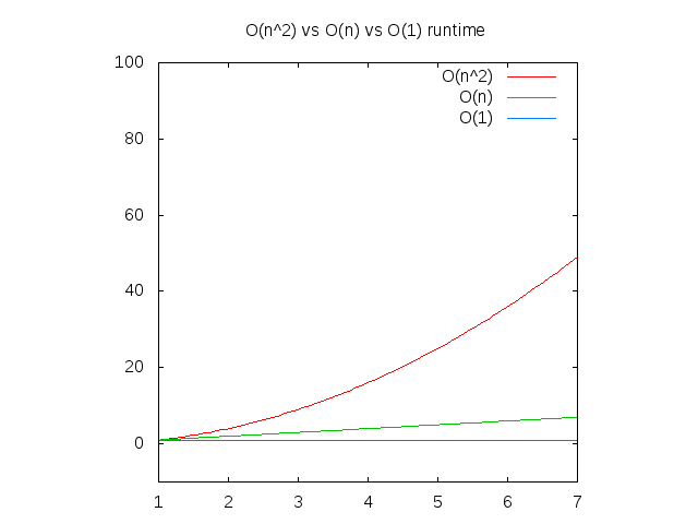 Here's a graph of the other major scales. You can see that at this scale, "constant time" and "logarithmic" seem very close:
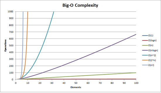
Here is the wiki page for "Big O": https://en.wikipedia.org/wiki/Big_O_notation
Constant time: O(1)
A function that does not grow in steps or operations as the input size grows is said to be running at constant time.
def sum_of_n_formula(n): return (n * (n + 1)) // 2 print(sum_of_n_formula(10))
That is, no matter how big n gets, the number of operations stays the same. "Constant time" growth is noted as O(1).
Linear growth: O(n)
The growth rate for the "range" solution to our earlier summing problem (repeated below) is known as linear growth.
With linear growth, as the input size (or in this case, the integer value) grows, the number of steps or operations grows at the same rate:
def sum_of_n_range(n): the_sum = 0 for i in range(1,n+1): the_sum = the_sum + i return the_sum print(sum_of_n_range(10))
Although there is another operation involved (the assignment of the_sum to 0), this additional step becomes trivial as the input size grows. We tend to ignore this step in our analysis because we are concerned with the function's growth, particularly as the input size becomes large. Linear growth is noted as O(n) where again, n is the input size -- growth of operations matching growth of input size.
Logarithmic growth: O(log(n))
A logarithm is an equation used in algebra. We can consider a log equation as the inverse of an exponential equation:
b^c = a ("b to the power of c equals a")
10³ = 1000 ## 10 cubed == 1000
is considered equivalent to: logba = c ("log with base b and value a equals c")
log101000 = 3
A logarithmic scale is a nonlinear scale used to represent a set of values that appear on a very large scale and a potentially huge difference between values, with some relatively small values and some exponentially large values. Such a scale is needed to represent all points on a graph without minimizing the importance of the small values. Common uses of a logarithmic scale include earthquake magnitude, sound loudness, light intensity, and pH of solutions. For example, the Richter Scale of earthquake magnitude grows in absolute intensity as it moves up the scale -- 5.0 is 10 times that of 4.0; 6.0 is 10 times that of 5.0; 7.0 is 10 times that of 6.0, etc. This is known as a base 10 logarithmic scale. In other words, a base 10 logarithmic scales runs as:
1, 10, 100, 1000, 10000, 100000, 1000000
Logarithms in Big O notation However, the O(log(n)) ("Oh log of n") notation refers to a base 2 progression - 2 is twice that of 1, 3 is twice that of 2, etc. In other words, a base 2 logarithmic scale runs as:
1, 2, 4, 8, 16, 32, 64
A classic binary search algorithm on an ordered list of integers is O(log(n)). You may recognize this as the "guess a number from 1 to 100" algorithm from one of the extra credit assignments.
def binary_search(alist, item): first = 0 last = len(alist)-1 found = False while first<=last and not found: midpoint = (first + last)//2 if alist[midpoint] == item: found = True else: if item < alist[midpoint]: last = midpoint-1 else: first = midpoint+1 return found print(binary_search([1, 3, 4, 9, 11, 13], 11)) print(binary_search([1, 2, 4, 9, 11, 13], 6))
The assumption is that the search list is sorted. Note that once the algorithm decides whether the search integer is higher or lower than the current midpoint, it "discards" the other half and repeats the binary searching on the remaining values. Since the number of loops is basically n/2/2/2/2, we are looking at a logarithmic order. Hence O(log(n))
Linear logarithmic growth: O(n * log(n))
The basic approach of a merge sort is to halve it; loop through half of it; halve it again.
def merge_sort(a_list): print(("Splitting ", a_list)) if len(a_list) > 1: mid = len(a_list) // 2 # (floor division, so lop off any remainder) left_half = a_list[:mid] right_half = a_list[mid:] merge_sort(left_half) merge_sort(right_half) i = 0 j = 0 k = 0 while i < len(left_half) and j < len(right_half): if left_half[i] < right_half[j]: a_list[k] = left_half[i] i = i + 1 else: a_list[k] = right_half[j] j = j + 1 k = k + 1 while i < len(left_half): a_list[k] = left_half[i] i = i + 1 k = k + 1 while j < len(right_half): a_list[k] = right_half[j] j = j + 1 k = k + 1 print(("Merging ", a_list)) a_list = [54, 26, 93, 17, 77, 31, 44, 55, 20] merge_sort(a_list) print(a_list)
The output of the above can help us understand what portions of the unsorted list are being managed:
('Splitting ', [54, 26, 93, 17, 77, 31, 44, 55, 20]) ('Splitting ', [54, 26, 93, 17]) ('Splitting ', [54, 26]) ('Splitting ', [54]) ('Merging ', [54]) ('Splitting ', [26]) ('Merging ', [26]) ('Merging ', [26, 54]) ('Splitting ', [93, 17]) ('Splitting ', [93]) ('Merging ', [93]) ('Splitting ', [17]) ('Merging ', [17]) ('Merging ', [17, 93]) ('Merging ', [17, 26, 54, 93]) ('Splitting ', [77, 31, 44, 55, 20]) ('Splitting ', [77, 31]) ('Splitting ', [77]) ('Merging ', [77]) ('Splitting ', [31]) ('Merging ', [31]) ('Merging ', [31, 77]) ('Splitting ', [44, 55, 20]) ('Splitting ', [44]) ('Merging ', [44]) ('Splitting ', [55, 20]) ('Splitting ', [55]) ('Merging ', [55]) ('Splitting ', [20]) ('Merging ', [20]) ('Merging ', [20, 55]) ('Merging ', [20, 44, 55]) ('Merging ', [20, 31, 44, 55, 77]) ('Merging ', [17, 20, 26, 31, 44, 54, 55, 77, 93]) [17, 20, 26, 31, 44, 54, 55, 77, 93]
Here's an interesting description comparing O(log(n)) to O(n * log(n)):
log(n) is proportional to the number of digits in n. n * log(n) is n times greater. Try writing the number 1000 once versus writing it one thousand times. The first takes O(log(n)) time, the second takes O(n * log(n) time. Now try that again with 6700000000. Writing it once is still trivial. Now try writing it 6.7 billion times. We'll check back in a few years to see your progress.
Quadratic growth: O(n^2;)
O(n²) growth can best be described as "for each element in the sequence, loop through the sequence". This is why it's notated as n².
def all_combinations(the_list): results = [] for item in the_list: for inner_item in the_list: results.append((item, inner_item)) return results print(all_combinations(['a', 'b', 'c', 'd', 'e', 'f', 'g']))
Clearly we're seeing n * n, so 49 individual tuple appends.
[('a', 'a'), ('a', 'b'), ('a', 'c'), ('a', 'd'), ('a', 'e'), ('a', 'f'), ('a', 'g'), ('b', 'a'), ('b', 'b'), ('b', 'c'), ('b', 'd'), ('b', 'e'), ('b', 'f'), ('b', 'g'), ('c', 'a'), ('c', 'b'), ('c', 'c'), ('c', 'd'), ('c', 'e'), ('c', 'f'), ('c', 'g'), ('d', 'a'), ('d', 'b'), ('d', 'c'), ('d', 'd'), ('d', 'e'), ('d', 'f'), ('d', 'g'), ('e', 'a'), ('e', 'b'), ('e', 'c'), ('e', 'd'), ('e', 'e'), ('e', 'f'), ('e', 'g'), ('f', 'a'), ('f', 'b'), ('f', 'c'), ('f', 'd'), ('f', 'e'), ('f', 'f'), ('f', 'g'), ('g', 'a'), ('g', 'b'), ('g', 'c'), ('g', 'd'), ('g', 'e'), ('g', 'f'), ('g', 'g')]
Exponential Growth: O(2^n)
Exponential denotes an algorithm whose growth doubles with each additon to the input data set.
One example would be the recursive calculation of a Fibonacci series
def fibonacci(num): if num <= 1: return num return fibonacci(num - 2) + fibonacci(num - 1) for i in range(10): print(fibonacci(i), end=' ')
Best Case, Expected Case, Worst Case
Case analysis considers the outcome if data is ordered conveniently or inconveniently.
For example, given a test item (an integer), search through a list of integers to see if that item's value is in the list. Sequential search (unsorted):
def sequential_search(a_list, item): pos = 0 found = False for test_item in a_list: if test_item == item: found = True break return found test_list = [1, 2, 32, 8, 17, 19, 42, 13, 0] print(sequential_search(test_list, 2)) # best case: found near start print(sequential_search(test_list, 17)) # expected case: found near middle print(sequential_search(test_list, 999)) # worst case: not found
Analysis: 0(n) Because the order of this function is linear, or O(n), case analysis is not meaningful. Whether the best or worst case, the rate of growth is the same. It is true that "best case" results in very few steps taken (closer to O(1)), but that's not helpful in understanding the function. When case matters Case analysis comes into play when we consider that an algorithm may seem to do well with one dataset (best case), not as well with another dataset (expected case), and poorly with a third dataset (worst case). A quicksort picks a random pivot, divides the unsorted list at that pivot, and sorts each sublist by selecting another pivot and dividing again.
def quick_sort(alist): """ initial start """ quick_sort_helper(alist, 0, len(alist) - 1) def quick_sort_helper(alist, first_idx, last_idx): """ calls partition() and retrieves a split point, then calls itself with '1st half' / '2nd half' indices """ if first_idx < last_idx: splitpoint = partition(alist, first_idx, last_idx) quick_sort_helper(alist, first_idx, splitpoint - 1) quick_sort_helper(alist, splitpoint + 1, last_idx) def partition(alist, first, last): """ main event: sort items to either side of a pivot value """ pivotvalue = alist[first] # very first item in the list is "pivot value" leftmark = first + 1 rightmark = last done = False while not done: while leftmark <= rightmark and alist[leftmark] <= pivotvalue: leftmark = leftmark + 1 while alist[rightmark] >= pivotvalue and rightmark >= leftmark: rightmark = rightmark - 1 if rightmark < leftmark: done = True else: # swap two items temp = alist[leftmark] alist[leftmark] = alist[rightmark] alist[rightmark] = temp # swap two items temp = alist[first] alist[first] = alist[rightmark] alist[rightmark] = temp return rightmark alist = [54, 26, 93, 17, 77] quick_sort(alist) print(alist)
Best case: all elements are equal -- sort traverses the elements once (O(n)) Worst case: the pivot is the biggest element in the list -- each iteration just works on one item at a time (O(n²)) Average case: the pivot is more or less in the middle -- O(n * log(n))
"order" analysis example
Let's take an arbitrary example to analyze. This algorithm is working with the variable n -- we have not defined n because it represents the input data, and our analysis will ask: how does the time needed change as n grows? However, we can assume that n is a sequence.
a = 5 # count these up: b = 6 # 3 statements c = 10 for k in range(n): w = a * k + 45 # 2 statements: v = b * b # but how many times # will they execute? for i in range(n): for j in range(n): x = i * i # 3 statements: y = j * j # how many times? z = i * j d = 33 # 1 statement
* We can count assignment statements that are executed once: there are 4 of these. * The 2 statements in the first loop are each being executed once for each iteration of the loop -- and it is iterating n times. So we call this 2n. * The 3 statements in the second loop are being executed n times * n times (a nested loop of range(n). We can call this n² ("n squared"). So the order equation can be expressed as 4 + 2n + n² eliminating the trivial factors However, remember that this analysis describes the growth rate of the algorithm as input size n grows very large. As n gets larger, the impact of 4 and of 2n become less and less significant compared to n²; eventually these elements become trivial. So we eliminate the lessor factors and pay attention only to the most significant -- and our final calculation is O(n²).
Big O Analysis: rules of thumb
Here are some practical ways of thinking, courtesy of The Idiot's Guide to Big O
* Does it have to go through the entire list? There will be an n in there somewhere. * Does the algorithms processing time increase at a slower rate than the size of the data set? Then there's probably a log(n) in there. * Are there nested loops? You're probably looking at n^2 or n^3. * Is access time constant irrelevant of the size of the dataset?? O(1)
More Big O recursion examples
These were adapted from a stackoverflow question. Just for fun(!) these are presented without answers; answers on the next page.
def recurse1(n): if n <= 0: return 1 else: return 1 + recurse1(n-1)
def recurse2(n): if n <= 0: return 1 else: return 1 + recurse2(n-5)
def recurse3(n): if n <= 0: return 1 else: return 1 + recurse3(n / 5)
def recurse4(n, m, o): if n <= 0: print('{}, {}'.format(m, o)) else: recurse4(n-1, m+1, o) recurse4(n-1, m, o+1)
def recurse5(n): for i in range(n)[::2]: # count to n by 2's (0, 2, 4, 6, 7, etc.) pass if n <= 0: return 1 else: return 1 + recurse5(n-5)
More Big O recursion examples: analysis
def recurse1(n): if n <= 0: return 1 else: return 1 + recurse1(n-1)
This function is being called recursively n times before reaching the base case so it is O(n) (linear)
def recurse2(n): if n <= 0: return 1 else: return 1 + recurse2(n-5)
This function is called n-5 for each time, so we deduct five from n before calling the function, but n-5 is also O(n) (linear).
def recurse3(n): if n <= 0: return 1 else: return 1 + recurse3(n // 2)
This function is log(n), for every time we divide by 2 before calling the function.
def recurse4(n, m, o): if n <= 0: print('{}, {}'.format(m, o)) else: recurse4(n-1, m+1, o) recurse4(n-1, m, o+1)
In this function it's O(2^n), or exponential, since each function call calls itself twice unless it has been recursed n times.
def recurse5(n): for i in range(n)[::2]: # count to n by 2's (0, 2, 4, 6, 7, etc.) pass if n <= 0: return 1 else: return 1 + recurse5(n-5)
The for loop takes n/2 since we're increasing by 2, and the recursion takes n-5 and since the for loop is called recursively, the time complexity is in (n-5) * (n/2) = (2n-10) * n = 2n^2- 10n, so O(n²)
Efficiency of core Python Data Structure Algorithms
note: "k" is the list being added/concatenated/retrieved
List Operation Big-O Efficiency index[] O(1) index assignment O(1) append O(1) pop() O(1) pop(i) O(n) insert(i,item) O(n) del operator O(n) iteration O(n) contains (in) O(n) get slice [x:y] O(k) del slice O(n) set slice O(n + k) reverse O(n) concatenate O(k) sort O(n * log(n) multiply O(nk)
A rundown of each structure and the O time to complete operations on each structure are noted here: https://wiki.python.org/moin/TimeComplexityDict Operation Big-O Efficiency (avg.) copy O(n) get item O(1) set item O(1) delete item O(1) contains (in) O(1) iteration O(n)
Common Algorithms Organized by Efficiency
O(1) time 1. Accessing Array Index (int a = ARR[5]) 2. Inserting a node in Linked List 3. Pushing and Poping on Stack 4. Insertion and Removal from Queue 5. Finding out the parent or left/right child of a node in a tree stored in Array 6. Jumping to Next/Previous element in Doubly Linked List and you can find a million more such examples... O(n) time 1. Traversing an array 2. Traversing a linked list 3. Linear Search 4. Deletion of a specific element in a Linked List (Not sorted) 5. Comparing two strings 6. Checking for Palindrome 7. Counting/Bucket Sort and here too you can find a million more such examples.... In a nutshell, all Brute Force Algorithms, or Noob ones which require linearity, are based on O(n) time complexity O(log(n)) time 1. Binary Search 2. Finding largest/smallest number in a binary search tree 3. Certain Divide and Conquer Algorithms based on Linear functionality 4. Calculating Fibonacci Numbers - Best Method The basic premise here is NOT using the complete data, and reducing the problem size with every iteration O(n * log(n)) time 1. Merge Sort 2. Heap Sort 3. Quick Sort 4. Certain Divide and Conquer Algorithms based on optimizing O(n^2) algorithms The factor of 'log(n)' is introduced by bringing into consideration Divide and Conquer. Some of these algorithms are the best optimized ones and used frequently. O(n^2) time 1. Bubble Sort 2. Insertion Sort 3. Selection Sort 4. Traversing a simple 2D array These ones are supposed to be the less efficient algorithms if their O(n * log(n)) counterparts are present. The general application may be Brute Force here.
Practice Problems
Practice Problem: List sum (linear and recursion)
Given a list of numbers, sum them up using a linear approach and using recursion. Answers appear on next slide.
Practice Problem: List sum (linear and recursion) (Answers)
Given a list of numbers, sum them up using a linear approach and using recursion. linear approach
def list_sum_linear(num_list): the_sum = 0 for i in num_list: the_sum = the_sum + i return the_sum print(list_sum([1,3,5,7,9]))
recursion approach
def list_sum_recursive(num_list): if len(num_list) == 1: return num_list[0] else: return num_list[0] + list_sum_recursive(num_list[1:]) print(list_sum_recursive([1,3,5,7,9]))
Practice Problems: ETL Developer
This was a question in an interview at AppNexus that I helped conduct, calling for a Python ETL developer (extract, transform, load) -- not a high-end position, but still one of value (and significant remuneration). Answers appear on next slide. Class and STDOUT data stream
class OT(object): def __init__(self, *thisfile): self.file = thisfile def write(self, obj): for f in self.file: f.write(obj) sys.stdout = OT(sys.stdout, open('myfile.txt'))
1. What does this code do? Feel free to talk it through 2. What is the 'object' in the parentheses? 3. What does the asterisk in *thisfile mean? local and global namespace
var = 10 def myfunc(): var = 20 print(var) myfunc() print(var)
1. What will this code output? Why? "sort" functions and multidimensional structures
def myfunc(arg): return arg struct = [ { 'a': [1, 2, 3], 'b': [4, 5, 6], 'c': [7, 8, 9] }, { 'a': [10, 12, 13], 'b': [1, 2, 3], 'c': [1, 2, 3] }, { 'a': [1, 2, 3], 'b': [1, 2, 3], 'c': [1, 2, 3] } ] dd = sorted(struct, key=myfunc)
1. What type of object is arg? 2. Rewrite the 'myfunc' function so the dicts are sorted by the sum of values associated with 'c'. 3. Convert your 'myfunc' function as a lambda 4. Loop through struct and print out just the last value of each list. import statements 1. which of these import statements do you favor and why?
import datetime import datetime as dt from datetime import *
Practice Problems: ETL Developer (Answers)
Class and STDOUT data stream
class OT(object): def __init__(self, *thisfile): self.file = thisfile def write(self, obj): for f in self.file: f.write(obj) sys.stdout = OT(sys.stdout, open('myfile.txt', 'w'))
1. What does this code do? Feel free to talk it through. The class creates an object that stores multiple open data streams (in this case, sys.stdout and an open filehandle) in an attribute of the instance. When the write() method is called on the object, the class will write to each of the stream(s) initialized in the instance, in this case to sys.stdout() and to the open file. The OT instance is being assigned to sys.stdout. This means that any call to sys.stdout.write() will pass to the instance. In addition, the print statement will also call sys.stdout.write(). The effect of this code is for any print statements that occur afterward to write to both STDOUT and to the filehandle initialized when the instance was constructed. 2. What is the 'object' in the parentheses? It causes the OT class to inherit from object. Thus OT is a new-style class. 3. What does the asterisk in *thisfile mean? It allows any number of arguments to be passed to the constructor / to __init__. local and global namespace
var = 10 def myfunc(): var = 20 print(var) myfunc() print(var)
1. What will this code output? Why? 20 10 Inside myfunc() the local variable var is set to 20 and printed. Once returned from the function, the global var is "revealed" (i.e., it is now accessible under the name var. "sort" functions and multidimensional structures
def myfunc(arg): return arg struct = [ { 'a': [1, 2, 3], 'b': [4, 5, 6], 'c': [7, 8, 9] }, { 'a': [10, 12, 13], 'b': [1, 2, 3], 'c': [1, 2, 3] }, { 'a': [1, 2, 3], 'b': [1, 2, 3], 'c': [1, 2, 3] } ] dd = sorted(struct, key=myfunc)
1. What type of object is arg? arg is a string, or a key from the dict. 2. Rewrite the 'myfunc' function so the dicts are sorted by the sum of values associated with 'c'. def myfunc(arg): return sum(myfunc(arg)) 3. Convert your 'myfunc' function as a lambda lambda arg: sum(myfunc(arg)) 4. Loop through struct and print out just the last value of each list. for key in struct: print(struct[key][-1]) import statements 1. which of these import statements do you favor and why?
import datetime import datetime as dt from datetime import *
The answer should see the candidate disavowing any use of the last form, which imports all symbols from the datetime module into the global namespace, and thus risks collisions with other modules
Practice Problems: Calculate a Factorial using linear approach and recursion
A factorial is the multiplication of each integer in a consecutive range starting at 0. So 4 factorial is 1 * 2 * 3 * 4 = 24. In the recursive approach, the function's job is very simply to multiply the number passed to it by the product produced by another call to the function with a number one less than the one passed to it. The function thus continues to call itself with one less integer until the argument becomes 0, at which point it returns. As each recursively called function returns, it passes back the value it was passed, multiplied by the value passed to it. So on the way back the values are multiplied. Answers appear on next slide.
Practice Problems: Calculate a Factorial using linear approach and recursion (Answers)
factorial: "linear" approach
def factorial_linear(n): prod = 1 for i in range(1, n+1): prod = prod * i return prod
factorial: "recursion" approach
def factorial_recursive(n): if n < 1: return 1 else: return_number = n * factorial_recursive(n-1) # recursive call print('{}! = {}'.format(n, return_number)) return return_number
Practice Problems: Calculate a fibonacci series using linear approach and recursion
A fibonacci series is one in which each number is the sum of the two previous numbers. Answers appear on next slide.
Practice Problems: Calculate a fibonacci series using linear approach and recursion (Answers)
A fibonacci series is one in which each number is the sum of the two previous numbers. linear approach
def fib_lin(max): prev = 0 curr = 1 while curr < max: print(curr, end=' ') newcurr = prev + curr prev = curr curr = newcurr
Practice Problems: Calculate prime numbers to a max value
Answers appear on next slide.
Practice Problems: Calculate prime numbers to a max value (Answer)
def get_primes(maxval): startval = 2 while startval <= maxval: counter = 2 while counter < startval: if startval % counter == 0: startval = startval + 1 counter = 2 continue else: counter = counter + 1 continue print(startval) startval = startval + 1
Practice Problems: reverse a sequence
this_list = ['a', 'b', 'c', 'd', 'e']
Answers appear on next slide.
Practice Problems: reverse a sequence (Answer)
this_list = ['a', 'b', 'c', 'd', 'e'] # using reversed print(list(reversed(this_list))) # using sorted print(sorted(this_list, reverse=True)) # using negative stride print(this_list[::-1]) # using list.insert() newlist = [] for el in this_list: newlist.insert(0 ,el) # using indices newlist = [] index = len(this_list)-1 while index >= 0: newlist.append(this_list[index]) index = index - 1
Practice Problems: given two strings, detect whether one is an anagram of the other
Answers appear on next slide.
Practice Problems: given two strings, detect whether one is an anagram of the other (Answer)
def ispalindrome(test1, test2): test2 = list(test2) for char in test1: try: test2.remove(char) except ValueError: return False if test2: return False return True str1 = 'allabean' str2 = 'beallana' print(ispalindrome('allabean', 'beallana')) print(ispalindrome('allabean', 'beallaaa'))
Practice Problems: given a string, detect whether it is a palindrome
Answers appear on next slide.
Practice Problems: given a string, detect whether it is a palindrome (Answer)
test_string = 'Able was I ere I saw Elba' if test_string.lower() == test_string.lower()[::-1]: print('"{}" is a palindrome'.format(test_string))
Python "gotcha" questions
These really are unfair, and not necessarily a good barometer -- they simply require that you know the quirks that lead to the strange output. But they can point out interesting aspects of the language. Answers appear on next slide. for each of the following blocks of code, what is the output?
def extendList(val, list=[]): list.append(val) return list list1 = extendList(10) list2 = extendList(123,[]) list3 = extendList('a') print("list1 = %s" % list1) print("list2 = %s" % list2) print("list3 = %s" % list3)
def multipliers(): return [lambda x : i * x for i in range(4)] print([m(2) for m in multipliers()])
class Parent(object): x = 1 class Child1(Parent): pass class Child2(Parent): pass print(Parent.x, Child1.x, Child2.x) Child1.x = 2 print(Parent.x, Child1.x, Child2.x) Parent.x = 3 print(Parent.x, Child1.x, Child2.x)
def div1(x,y): print("%s/%s = %s" % (x, y, x/y)) def div2(x,y): print("%s//%s = %s" % (x, y, x//y)) div1(5,2) div1(5.,2) div2(5,2) div2(5.,2.)
1. list = [ [ ] ] * 5 2. list # output? 3. list[0].append(10) 4. list # output? 5. list[1].append(20) 6. list # output? 7. list.append(30) 8. list # output?
Python "gotcha" questions (Answers)
for each of the following blocks of code, what is the output?
def extendList(val, list=[]): list.append(val) return list list1 = extendList(10) list2 = extendList(123,[]) list3 = extendList('a') print("list1 = %s" % list1) print("list2 = %s" % list2) print("list3 = %s" % list3) # [10, 'a'] # [123] # [10, 'a']
default list is constructed at time of definition
def multipliers(): return [lambda x : i * x for i in range(4)] print([m(2) for m in multipliers()]) # [6, 6, 6, 6]
Python closures are late binding, means that when we finally call the function it will look up the value of i and find a 6
class Parent(object): x = 1 class Child1(Parent): pass class Child2(Parent): pass print(Parent.x, Child1.x, Child2.x) Child1.x = 2 print(Parent.x, Child1.x, Child2.x) Parent.x = 3 print(Parent.x, Child1.x, Child2.x) ## 1 1 1 ## 1 2 1 ## 3 2 3
Attribute lookup starts in instance, then checks class and then parent class(es).
def div1(x,y): print("%s/%s = %s" % (x, y, x/y)) def div2(x,y): print("%s//%s = %s" % (x, y, x//y)) div1(5,2) div1(5.,2) div2(5,2) div2(5.,2.) ## 2 ## 2.5 ## 2 ## 2
"floor division" (i.e., integerized result) is the default with integer operands; also can be specified with the // "floor division" operator
1. list = [ [ ] ] * 5 2. list # output? 3. list[0].append(10) 4. list # output? 5. list[1].append(20) 6. list # output? 7. list.append(30) 8. list # output? ## [[], [], [], [], []] ## [[10], [10], [10], [10], [10]] ## [[10, 20], [10, 20], [10, 20], [10, 20], [10, 20]] ## [[10, 20], [10, 20], [10, 20], [10, 20], [10, 20], 30]
key: in a * multiplication, Python simply duplicates the reference rather than the list
[advanced] Functional Programming
Functional Programming: Overview
We may say that there are three commonly used styles (sometimes called paradigms) of program design: imperative/procedural, object-oriented and functional. Here we'll tackle a common problem (summing a sequence of integers, or an arithmetic series) using each style: imperative or procedural involves a series of statements along with variables that change as a result. We call these variable values the program's state.
mysum = 0 for counter in range(11): mysum = mysum + counter print(mysum)
object-oriented uses object state to produce outcome.
class Summer(object): def __init__(self): self.sum = 0 def add(self, num): self.sum = self.sum + num s = Summer() for num in range(11): s.add(num) print(s.sum)
functional combines pure functions (functions that do not touch outside variables, but only work with arguments and return values) to produce outcome. No state change is involved.
print(sum(range(11)))
A pure function is one that only handles input, output and its own variables -- it does not affect nor is it affected by global or other variables existing outside the function. Because of this "air-tightness", functional programming can be tested more reliably than the other styles. Some languages are designed around a single style or paradigm. But since Python is a "multi-paradigm" language, it is possible to use it to code in any of these styles. To employ functional programming in our own programs, we need only seek to replace imperative code with functional code, combining pure functions in ways that replicate some of the patterns that we use to iterate, summarize, compute, etc. After some experience coding in this style, you may recognize patterns for iteration, accumulation, etc. and more readily employ them in your programs, making them more predictable, testable and less prone to error. Note: Python documentation provides a solid overview of functional programming in Python.
Mary Rose Cook provides a plain language introduction to functional programming.
O'Reilly publishes a free e-book with a comprehensive review of functional programming by Python luminary David Mertz.
Review: lambdas
Lambda functions are simply inline functions -- they can be defined entirely within a single statement, within a container initialization, etc.
Lambdas are most often used inside functions like sorted():
# sort a list of names by last name names = [ 'Josh Peschko', 'Gabriel Feghali', 'Billy Woods', 'Arthur Fischer-Zernin' ] sortednames = sorted(names, key=lambda name: name.split()[1]) # sort a list of CSV lines by the 2nd column in the file slines = sorted(lines, lambda x: x.split(',')[2])
We will see lambdas used in other functions such as map(), filter() and reduce().
Review: list comprehensions; set comprehensions and dict comprehensions
List, set and dict comprehensions can filter or transform sequences in a single statement.
Functional programming (and algorithms in general) often involves the processing of sequences. List comprehensions provide a flexible way to filter and modify values within a list.
list comprehension: return a list
nums = [1, 2, 3, 4, 5] dblnums = [ val * 2 for val in nums ] print(dblnums) # [2, 4, 6, 8, 10] print([ val * 2 for val in nums if val > 2]) # [6, 8, 10]
set comprehension: return a set
states = { line.split(':')[3] for line in open('student_db.txt').readlines()[1:] }
dict comprehension: return a dict
student_states = { line.split(':')[0]: line.split(':')[3] for line in open('student_db.txt').readlines()[1:] }
map() and filter() as alternatives to list comprehensions
lthough list comprehensions have nominally replaced map() and filter(), these functions are still used in many functional programming algorithms.
map(): apply a transformation function to each item in a sequence
# square some integers sqrd = [x ** 2 for x in range(6)] # [1, 4, 9, 16, 25] # get string lengths lens = list(map(len, ['some', 'words', 'to', 'get', 'lengths', 'from'])) print(lens) # [4, 5, 2, 3, 7, 4]
filter(): apply a filtering function to each item in a sequence
pos = [x for x in [-5, 2, -3, 17, 6, 4, -9] if x > 0] print(pos) # [2, 17, 6, 4]
reduce() for accumulation of values
Like map() or filter(), reduce() applies a function to each item in a sequence, but accumulates a value as it iterates.
It accumulates values through a second variable to its processing function. In the below examples, the accumulator is a and the current value of the iteration is x. a grows through the accumulation, as if the function were saying a = a + x or a = a * x.
Here is our arithmetic series for integers 1-10, done with reduce():
from functools import reduce def addthem(a, x): return a + x intsum = reduce(addthem, list(range(1, 11))) # same using a lambda intsum = reduce(lambda a, x: a + x, list(range(1, 11)))
Just as easily, a factorial of integers 1-10:
from functools import reduce facto = reduce(lambda a, x: a * x, list(range(1, 11))) # 3628800
default value
Since reduce() has to start with a value in the accumulator, it will attempt to begin with the first element in the source list. However, if each value is being transformed before being accumulated, the first computation may result in an error:
from functools import reduce strsum = reduce(lambda a, x: a + int(x), ['1', '2', '3', '4', '5']) # TypeError: cannot concatenate 'str' and 'int' objects
This is apparently happening because python is trying to add int('1') to '' (i.e., reduce() does not see the transform and so uses an 'empty' version of the type, in this case an empty string).
In these cases we can supply an initial value to reduce(), so it knows where to begin:
from functools import reduce strsum = reduce(lambda a, x: a + int(x), ['1', '2', '3', '4', '5'], 0)
Higher-Order Functions Any function that takes a function as an argument, or that returns a function as a return value, is a higher-order function. map(), filter(), reduce(), sorted all take functions as arguments. @properties, @staticmethod, @classmethod all take a given function as argument and return a modified function as a return value.
any() and all(): return True based on truth of elements
any(): return True if any elements are True
any([1, 0, 2, 0, 3]) # True: at least one item is True any([0, [], {}, '']) # False: none of the items is True
all(): return True if all elements are True
all([1, 5, 0.0001, 1000]) # True: all items are True all([1, 5, 9, 10, 0, 20]) # False: one item is not True
generators
Generators are iterators that can calculate and generate any number of items.
Generators behave like iterators, except that they yield a value rather than return one, and they remember the value of their variables so that the next time the class' next() method is called, it picks up where the last left off (at the point of yield). . As a generator is an iterator, next() calls the function again to produce the next item; and StopIteration causes the generator to stop iterating. (next() is called automatically by iterators like for.
Generators are particularly useful in producing a sequence of n values, i.e. not a fixed sequence, but an unlimited sequence. In this example we have prepared a generator that generates primes up to the specified limit.
def get_primes(num_max): """ prime number generator """ candidate = 2 found = [] while True: if all(candidate % prime != 0 for prime in found): yield candidate found.append(candidate) candidate += 1 if candidate >= num_max: raise StopIteration my_iter = get_primes(100) print(next(my_iter)) # 2 print(next(my_iter)) # 3 print(next(my_iter)) # 5 for i in get_primes(100): print(i)
[pr]
(base) david@192 repos % git clone git@github.com:davidostest/demo_20230808.git
If this is the first time connecting to git, git responds with the following prompt:
Cloning into 'demo_20230808'...
The authenticity of host 'github.com (140.82.113.4)' can't be established.
ECDSA key fingerprint is SHA256:p2QAMXNIC1TJYWeIOttrVc98/R1BUFWu3/LiyKgUfQM.
Are you sure you want to continue connecting (yes/no/[fingerprint])? yes
Type yes and hit [Enter]. This creates a special .git directory here. You'll see a message to this effect.
(Note that if you see a DNS SPOOFING/DOING SOMETHING NASTY warning, you may need to delete the github.com line from your known_hosts file. Let me know if you're not sure what to do in this case.)
User-Defined Functions
Introduction: User-Defined Functions
A user-defined function is a named code block -- very simply, a block of Python code that we can call by name. These functions are used and behave very much like built-in functions, except that we define them in our own code.
def addthese(val1, val2): # function definition; argument signature
valsum = val1 + val2
return valsum # return value
x = addthese(5, 10) # function call; 2 arguments passed;
# return value assigned to x
print(x) # 15
There are two primary reasons functions are useful: to reduce code duplication and to organize our code: Reduce code duplication: a named block of code can be called numerous times in a program, which means the same series of statements can be executed repeatedly, without having to type them out multiple times in the code. Organize code: large programs can be difficult to read, even with helpful comments. Dividing code into named blocks allows us to identify the major steps our code can take, and see at a glance what steps are being taken and the order in which they are taken. We have learned about using simple functions for sorting; in this unit we will learn about: 1) different ways to define function arguments 2) the "scoping" of variables within functions 3) the four "naming" scopes within Python
Review: functions are named code blocks
The block is executed every time the function is called.
def print_hello():
print("Hello, World!")
print_hello() # prints 'Hello, World!'
print_hello() # prints 'Hello, World!'
print_hello() # prints 'Hello, World!'
When we run this program, we see the greeting printed three times.
Review: function argument(s)
Any argument(s) passed to a function are aliased to variable names inside the function definition.
def print_hello(greeting, person): # 2 strings aliased to objects
# passed in the call
full_greeting = f"{greeting}, {person}!"
print(full_greeting)
print_hello('Hello', 'World') # pass 2 strings: prints "Hello, World!"
print_hello('Bonjour', 'Python') # pass 2 strings: prints "Bonjour, Python!"
print_hello('squawk', 'parrot') # pass 2 strings: prints "squawk, parrot!"
Review: the return statement returns a value
Object(s) are returned from a function using the return statement.
def print_hello(greeting, person):
full_greeting = greeting + ", " + person + "!"
return full_greeting
msg = print_hello('Bonjour', 'parrot') # full_greeting
# aliased to msg
print(msg) # 'Bonjour, parrot!'
Multi-target Assignment
This convenience allows us to assign values in a list to individual variable names.
line = 'Acme:23.9:NY'
items = line.split(':')
print(items) # ['Acme', '23.9', 'NY']
name, revenue, state = items
print(revenue) # 23.9
This kind of assignment is sometimes called "unpacking" because it assigns a container of items to individual variables.
We can assign multiple values to multiple variables in one statement too:
name, revenue, state = 'Acme', '23.9', 'NY'
(The truth is that the 3 values on the right comprise a tuple even without the paretheses, so we are technically still unpacking.)
If the number of items on the right does not match the number of variables on the left, an error occurs:
mylist = ['a', 'b', 'c', 'd']
x, y, z = mylist # ValueError: too many values to unpack
v, w, x, y, z = mylist # ValueError: not enough values to unpack
We also see multi-target assignment when returning multiple values from a function:
def return_some_values():
return 10, 20, 30, 40
a, b, c, d = return_some_values()
print(a) # 10
print(d) # 40
This means that like with standard unpacking, the number of variables to the right of a function call must match the number of values returned from the function call.
Summary argument types: positional and keyword
Your choice of type depends on whether they are required.
positional: args are required and in particular order
def sayname(firstname, lastname):
print(f"Your name is {firstname} {lastname}")
sayname('Joe', 'Wilson') # passed two arguments: correct
sayname('Joe') # TypeError: sayname() missing 1 required positional argument: 'lastname'
keyword: args are not required, can be in any order, and the function specifies a default value
def sayname(lastname, firstname="Citizen"):
print(f"Your name is {firstname} {lastname}")
sayname('Wilson', firstname='Joe') # Your name is Joe Wilson
sayname('Wilson') # Your name is Citizen Wilson
Variable name scoping inside functions
Variable names initialized inside a function are local to the function, and not available outside the function.
def myfunc():
a = 10
return a
var = myfunc() # var is now 10
print(a) # NameError ('a' does not exist here)
Note that although the object associated with a is returned and assigned to var, the name a is not available outside the function. Scoping is based on names.
global variables (i.e., ones defined outside a function) are available both inside and outside functions:
var = 'hello global'
def myfunc():
print(var)
myfunc() # hello global
The four variable scopes: (L)ocal, (E)nclosing, (G)lobal and (B)uiltin
Variable scopes "overlay" one another; a variable can be "hidden" by a same-named variable in a "higher" scope.
From top to bottom: